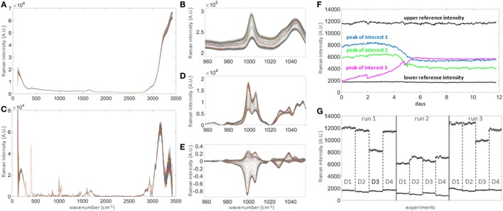
Figure 3.

Raman signal processing for untargeted univariate data analysis. (A) 300 raw spectra collected hourly over 12 days in one bioreactor. (B) Magnified spectral region between wavenumbers 960 and 1,050, showing clear shift of signal baseline over time. The shift over time is of similar magnitude as most prominent peaks and hence needs to be corrected in order to quantify genuine changes of Raman intensity, such as seen in the subtle non-parallel patterns on the left-hand side of the right peak. (C) Baseline-corrected spectra. The correction highlights the potential peaks of interest. (D) Same region as in (B) after correction, demonstrating that the spectra are significantly re-aligned. (E) Same as (D) after subtracting the averaged first two spectra, in order to normalize the signals to t = 0 and highlighting true signal fluctuations over time. (F) Example of time series for three peaks of interest (colored) showing patterns consistent with expected biochemical changes in the culture medium. As the intensity scale is not calibrated to a standard, two reference intensities consisting of the averages of three peaks with either constant high (at 292, 295, and 2,926 cm⁻¹) or low (at 324, 564, and 1,483 cm⁻¹) intensities over time (labeled “upper reference intensity” and “lower reference intensity,” respectively, the bold black lines showing the averages of both groups) were selected to perform internal signal normalization. This approach was used to normalize all time series between runs. (G) Comparison of reference time series between all runs and all donors (labeled D1–D4). This graph illustrates the unpredictable extensive probe-to-probe variability observed with this technology in this context, whether technical or biological, and the need for signal calibration or normalization to obtain comparable datasets between different bioreactors and experiments.