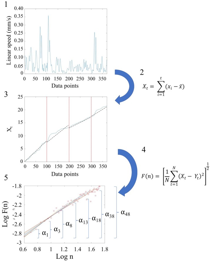
Figure 2.

Schematic steps to perform the Detrended Fluctuation Analysis (DFA) using the linear and angular speed profiles of the involuntary hear excursions. (Step 1) Sample raw linear speed data extracted from linear positional displacements of the head along the x-, y-, and z-axis. The magnitude of the rate of displacements frame by frame (the linear speed temporal profile) is obtained and the profile resampled at 2 Hz. The data is truncated to 370 points for all participants to ensure equal number of points (see Figure S1); (Step 2) Given the time series of length N = 370, (the minimum number of points across the data set) we obtain the integration or summation within 100-point window for each $X_t=\sum _{i=1}^t(x_i-\langle x\rangle )$ where t denotes the size of the window, x_i is each point in the series within the window and 〈x〉 is the overall mean across the entire time series with linear speed (empirical range bounded between 4.28e-05 and 10.14 mm/s over the entire data set.) The X_t is the cumulative sum or profile and the summation converts from a bounded time series to unbounded process. (Step 3) The cumulative profile X_t is divided into non-overlapping time windows of equal length n (range 4 ≤ n ≤ N/10) where N is the total number of points in the signal, which in our case is N = 370 (Chen et al., 2002). In each interval, a local least-squares straight-line fit (which is the local trend) is obtained using minimization of the least squares errors in each window. The resulting piecewise sequence of straight line fits is denoted Y_t, then we calculate the root-mean-square deviation from the trend, i.e., the fluctuation: $F(n)=\sqrt{\frac{1}{N}\sum _{t=1}^N{(X_t-Y_t)}^2}$. (Step 4) The above process of detrending and obtaining the fluctuation metric is repeated over a range of different window sizes and a log-log map of n vs. F(n) obtained. This map provides a relationship between F(n), the average fluctuation as a function of box size, and the box size n. As explained in (Peng et al., 1995a), the straight line of this log-log relation indicates statistical self-affinity expressed by the scaling exponent alpha, F(n) ∝ n^α. The exponent alpha (a generalization of the Hurst exponent Hurst, 1951, is a measure of long time memory in a time series) is the slope of the straight line fit to the log(n) vs. log(F(n)) relation using least squares. (Step 5) To obtain a series of alpha values for each participant, we windowed the data starting with 3 points, then 4 points, then 5 points, etc. to the maximum number of points (370) we had.