A note on Kalman Filter

Abstract

The Kalman Filter commonly employed by control engineers and other physical scientists has been successfully used in such diverse areas as the processing of signals in aerospace tracking and underwater sonar, and statistical quality control. More recently, it has been used in some nonengineering applications such as short-term forecasting, time series, survival analysis, and so on. In all of these situations, we have a set of equations governing the true state of a system and another set connecting the observations made at any given time on the system with its true state. The problem is that of predicting the true state of the system at any given time point based on available observations. The solution proposed in the vast literature of the subject depends on the assumptions made on the initial state of the system. In this paper, a method that is independent of the initial state is proposed. This is useful when the a priori information on the initial state is not available. The method is also applicable when some observations are missing.

1. Dynamical and Observational Equation

There is extensive literature on Kalman Filtering (KF) and its applications arising out of the seminal contributions by Kalman (1) and Kalman and Bucy (2).

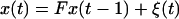
The general problem can be stated as follows. We have a time sequence of p and q-vector valued random variables {x(t), y(t)}, t = 1, 2, … related through structural equations

1.1

1.2

where F and H are p × p and q × p matrices, respectively, and the following hold, where E stands for expectation and C for covariance.

1.3

We have observations only on y(1), … , y(t) up to time t, and the problem is to estimate x(s) given y(1), … , y(t), or a subset of them.

In the engineering literature, estimation of x(t) is called smoothing if s < t, filtering if s = t, and prediction if s > t. An excellent review of KF and its applications to a wide variety of statistical problems can be found in refs. 1–5.

In the literature on KF, the conditions are usually stated in terms of independence of the variables involved instead of zero correlations as stated in 1.3. If we are interested in linear estimates of observations, we need only require the knowledge of the variances and covariances of the variables involved.

The theory described in the paper can be extended to the case where the matrices F and H in 1.1 and 1.2 and V and W in 1.3 depend on time.

2. Reduction to Linear Equations

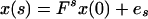
From 1.1,

2.1

with e_t = F_tξ_t, where

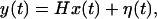
and I_p is the identity matrix of order p. A simple calculation yields

2.2

where I_s ⊗ V is the Kronecker product, and 0 is a null matrix of appropriate order.

From 1.2,

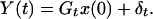
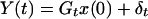
2.3

where δ(t) = He_t + η(t). A simple calculation gives

2.4

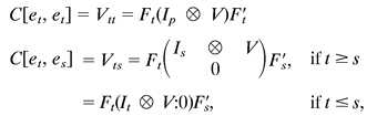
Writing Y′(t) = (y′(1), … , y′(t)) and

we have the composite linear model for observations up to time t

2.5

To estimate x(s) given Y(t) for any s and t, we need to consider the equations

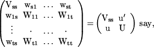
2.6

with the variance-covariance matrix of (e_s, δ_t),

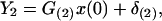
2.7

where V_ss, w_rs, and W_ij are as defined in 2.2 and 2.4, and u′ = (w_s1, … , w_st) and U = (W_ij).

3. Different Assumptions on x(0)

3.1. Given Prior Distribution of x(0).

Let x(0) have a prior mean μ and variance-covariance matrix P. Then we can write the model 2.6 as

3.1

with

3.2

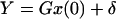
Then, using the least squares theory (ref. 6, pp. 544–547), the estimate of x(s) is

3.3

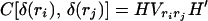
with the minimum dispersion error matrix

3.4

3.2. x(0) Is a Known Constant μ.

The solution in this case is the same as 3.4 with P in 3.2 replaced by the null matrix. Then the estimate of x(s) is

3.5

with the minimum error dispersion matrix

If x(0) is a constant, but its value is not known, then we may estimate x(0) from the second equation in 2.6 using least squares theory provided the rank of G_t is p. In such a case, the least squares estimate of x(0) is

3.6

Substituting x̂(0) for μ in 3.5, we have the empirical estimate

3.7

The estimate 3.7 and its dispersion matrix are derived in a more natural way in the next section.

3.3. No Information Is Available on x(0).

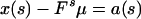
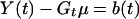
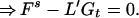
Consider a linear function L′Y(t) as an estimate of x(s) such that

3.8

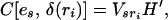
The variance-covariance matrix of x(s) − L′Y(t) is

3.9

where V_ss, u, and U are as defined in 2.7.

The minimum value of 3.9 subject to 3.8 is attained at

3.10

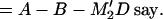
giving the same expression for the estimate of x(s) as the empirical estimate derived in 3.7. The minimum dispersion error matrix is

3.11

The second expression in 3.11 is the extra error due to the imposed condition 3.8. We call the estimate L′_*Y(t) the constrained linear predictor (CLP) of x(s).

We prove the following result, which will be used in Section 4. Let M be a matrix such that E(M′Y(t)) = 0 independently of x(0), which implies that M′G_t = 0. Then, with L_* as defined in 3.10,

3.12

4. Recursive Estimation

In the application of KF, it is customary to estimate x(s) using the available observations (y′(1), … , y′(r)) = Y′₁ (say), up to a time point r, and update the estimate when additional observations (y′(r + 1), … , y′(t)) = Y′₂ (say) are acquired. The methodology of such recursive estimation is well known in KF theory when unconstrained estimates (such as those discussed in Sections 3.1 and 3.2) are used.

We develop a similar method when CLPs as derived in Section 3.3 are required.

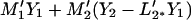
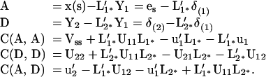
Let L′_1*Y₁ be the CLP of x(s) based on Y₁, and L′_2*Y₁ be the CLP of Y₂ based on Y₁. We consider a general linear function of Y₁, Y₂

4.1

and its deviation from x(s) as

4.2

The condition of unbiasedness of 4.1 independently of x(0) implies E(B) = 0, since E(A) and E(C) = 0. Then by the Condition 3.12,

4.3

Hence

4.4

The second term in 4.4 vanishes if we choose M₁ = L_1*. The best choice of M₂ which minimizes the first term is

4.5

To derive explicit expressions for A, D and their covariance, we write the basic linear model 2.6 by splitting Y(t) into the two components Y₁ and Y₂.

4.6

where G₍₁₎, G₍₂₎ are partitions of G_t and  δ₍₁₎, δ₍₂₎ are partitions of δ_t. The corresponding covariance matrix of x(s), Y₁, Y₂ is

4.7

obtained by partitioning the matrices u and U in 2.7.

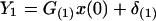
Using the formula 3.10, the CLP of x(s) based on Y₁ is

4.8

The CLP of Y₂ based on Y₁ is

4.9

Then

4.10

The updated CLP of x(s) is

4.11

with the minimum dispersion error

4.12

Note 1: The second equation in 2.6 is in the form of a mixed linear model, which enables us to estimate x(0), and also the matrices V and W if they are unknown by using MINQE method described in ref. 7.

Note 2: The linear model 2.6 is used when we want to estimate x(s) based on the data y(1), … , y(t). A more general problem is the estimation of x(s) based on y(r₁), … , y(r_n), observations made at n time points r₁, … , r_n. A particular situation is when observations on y are missing at certain time points, or some observations on y are discarded as not reliable or outliers. The linear equations appropriate for this is

4.13

where

where V_ij are as defined in 2.2. Then the general methods of Sections 3 and 4 apply.

Abbreviations

KF

Kalman Filter

CLP

constrained linear predictor

References

1.Kalman R E. J Basic Eng. 1960;82:34–45. [Google Scholar]
2.Kalman R E, Bucy R S. J Basic Eng. 1961;83:95–108. [Google Scholar]
3.Meinhold R J, Singpurwalla N D. Am Stat. 1983;37:123–127. [Google Scholar]
4.Meinhold R J, Singpurwalla N D. Am Stat. 1987;41:101–106. [Google Scholar]
5.Rao C R, Toutenburg H. Linear Models: Least Squares and Alternatives. 2nd Ed. New York: Springer; 1999. [Google Scholar]
6.Rao C R. Linear Statistical Inference and Its Applications. New York: Wiley; 1973. [Google Scholar]
7.Rao C R, Kleffe J. Estimation of Variance Components and Its Applications. Amsterdam: North–Holland; 1988. [Google Scholar]