Figure 3. Microscopic food flow.

(a) The distributions of interaction volumes from foragers to non-forager recipients, at seven ranges of recipient crop loads, follow an exponential probability density function of the form $p(v|c)={\lambda }_c{e}^{-{\lambda }_{c}v}$ (Equation 5, Figure 3—figure supplement 1). Here the seven rate parameters of the distributions (${\lambda }_c$) are plotted as a function of the recipient’s crop load ($c_{recipient}$). Mean $\pm$ STD of ${\lambda }_c$ are over different binnings of the histograms to which the exponential distribution function was fit (17 histogram binwidths uniformly covering the range [0.01–0.09]). Curve represents a fit of the function ${\lambda }_c=\frac{{\lambda }_0}{C_0-c}$ (Equation 6): ${\lambda }_0=7.01$, $C_0=1.14$, $R^2=0.93$. (b) Similarly to panel a, the rate parameters of the exponential distributions of interaction volumes were obtained for seven ranges of forager crop loads (Figure 3—figure supplement 2) and plotted as a function of the forager’s crop load, $c_{forager}$. Dashed curve represents a fit of the form ${\lambda }_c=\frac{const}{c_{forager}}$, similar to Equation 6, but instead of a fraction of the recipient’s empty crop space, ${\lambda }_c$ is assumed to be a fraction of the forager’s crop load. $R^2$ was negative, indicating that this function is no better fit to the data than a constant (solid line). (c) The distributions of ‘relative interaction volumes’, $\tilde{v}$, wherein each interaction volume was normalized to the available space in the receiver’s crop ($\tilde{v}=\frac{v}{C_0-c}$). The distributions collapse onto a single exponential function $p(\tilde{v})=\frac{1}{\lambda }{e}^{-\frac{1}{\lambda }\tilde{v}}$, $\lambda =0.12$, $R^2=0.96$. (d) The crop loads of non-foragers at interactions with foragers (blue, n as in b) compared to crop loads of all non-foragers in the colony (red, n = 202 per colony state bin). The distributions of crop loads at each colony state are plotted as a violin plot, and the mean $\pm$ SEM are plotted in solid lines. All panels in this figure represent pooled data from all three observation experiments. Source file is available in the Figure 1—source data 1.

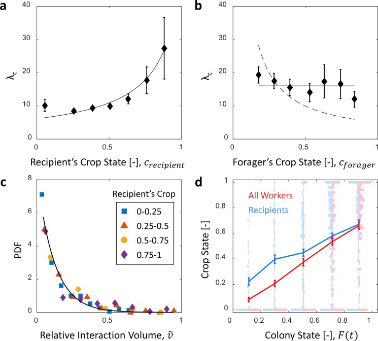
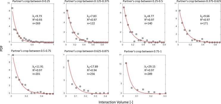
Figure 3—figure supplement 1. Interaction volume distributions given recipient crop load.

Each plot depicts a PDF of interaction volumes for a different range of recipient crop loads (indicated in the titles). Data was extracted from pooled data from all three observation experiments. All distributions were fit with exponentials as specified in the text (red curves). The fitted coefficients, $R^2$ of each fit, and sample sizes are indicated on the plots. See Methods section for details on units of food volume. To ensure that this procedure was not sensitive to histogram binwidths, it was performed on a range of binwidths as specified in the caption of Figure 3a. Here we show the results for a binwidth of 0.04.

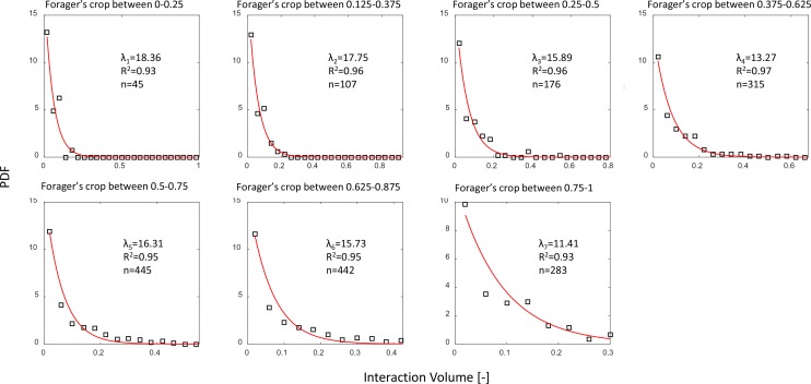
Figure 3—figure supplement 2. Interaction volume distributions given Forager’s crop load.

Each plot depicts a PDF of interaction volumes for a different range of forager crop loads (indicated in the titles). Data was extracted from all three observation experiments. All distributions were fit with exponentials as specified in the text (red curves). The fitted coefficients, $R^2$ of each fit, and sample sizes are indicated on the plots. See Methods section for details on units of food volume. To ensure that this procedure was not sensitive to histogram binwidths, it was performed on a range of binwidths as specified in the caption of Figure 3a. Here we show the results for a binwidth of 0.04.

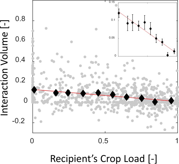
Figure 3—figure supplement 3. Mean interaction volumes as a function of the recipient’s crop load.

Interaction volumes (gray, pooled data from all three observation experiments) were binned according to the recipient’s crop load (black, mean $\pm$ SEM, n = 172,44,43,59,64,70,85,100,112,123 for bins 1–10, respectively) and fit with a function of the form $y=ax+b$ (red). Binned data and fit are magnified in the inset. The same fit was obtained for 5–10 bins, resulting in $a=-0.12$ and $b=0.13$ with $R^2=0.93,0.94,0.94,0.94,0.9,0.88$, respectively.