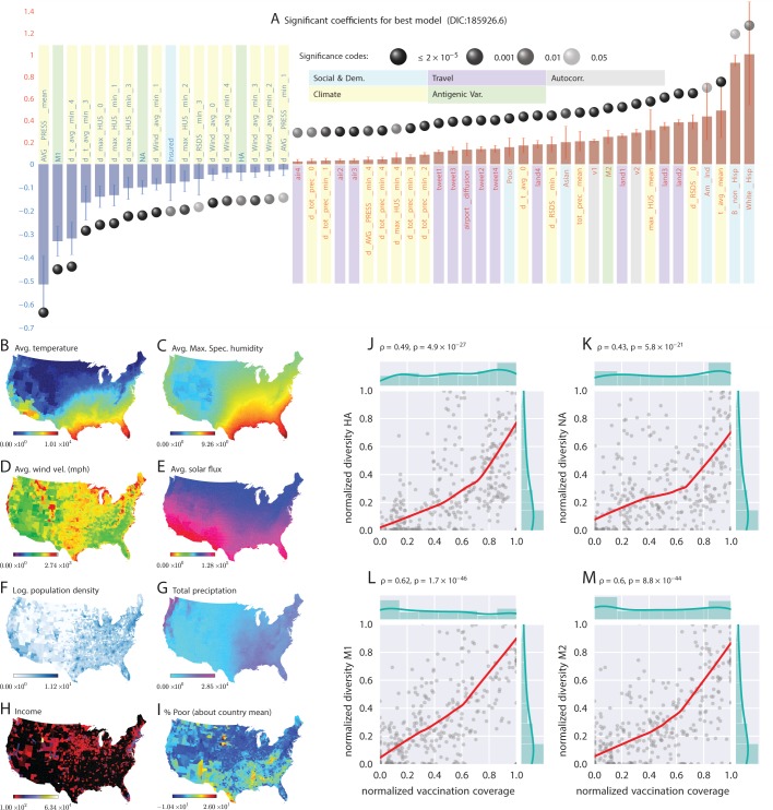
Figure 1. Putative determinants of seasonal influenza onset in the continental US and Poisson mixed-effect regression analysis (Approach 2).

Plate A shows the significant variables along with their computed influence coefficients from the mixed-effect Poisson regression analysis (the best model chosen from $\mathrm{126}$ different regression equations with different variable combinations). The statistically significant estimates of fixed effects are grouped into several classes: climate variables, economic and demographic variables, auto-regression variables, variables related to travel, and those related to antigenic diversity (see the last entry in Table 5 for the detailed regression equation used. The complete list of all models considered is given in Table S-D7). The fixed-effect regression coefficients plotted in Plate A are shown on a logarithmic scale, meaning that the absolute magnitude of predictor-specific effect is obtained by exponentiating the parameter value. A negative coefficient for a predictor variable suggests that the influenza rate falls as this factor increases, while a positive coefficient predicts a growing rate of infection as the parameter value grows. The integrated influence of individual predictors, under this model, is additive with respect to the county-specific rate of infection. For example, a coefficient of $\mathrm{-}\mathrm{0.6}$ for parameter AVG_PRESS_mean tells us that the average atmospheric pressure has a negative association with the influenza rate. As the mean atmospheric pressure for the county grows, the probability that the county would participate in an infection initiation wave falls. As $\exp \mathrm{}\mathrm{(}\mathrm{-}\mathrm{0.6}\mathrm{)}\mathrm{=}\mathrm{0.54}$, the rate of infection drops by $\mathrm{46}\mathrm{\%}$ when atmospheric pressure increases by one unit of zero-centered and standard-deviation-normalized atmospheric pressure. Similarly, an increase in the share of a white Hispanic population predicts an increase in influenza rate: A coefficient of 1.3 translates into a $\exp \mathrm{}\mathrm{(}\mathrm{1.3}\mathrm{)}\mathrm{\times }\mathrm{100}\mathrm{\%}\mathrm{-}\mathrm{100}\mathrm{\%}\mathrm{=}\mathrm{267}\mathrm{\%}$ rate increase, possibly, because of the higher social network connectivity associated with this segment of population. Plates B - I enumerate the average spatial distribution of a few key significant factors considered in Poisson regression: (B) average temperature; (C) average maximum specific humidity; (D) average wind velocity in miles per hour; (E) average solar flux; (F) logarithm of population density (people per square mile); (G) total precipitation; (H) income, and; (I) percent of poor as deviations about the country average. Plates J-M show the strong dependence between our estimated antigenic diversity (normalized, see Definition in text) corresponding to the HA, NA, M1, and M2 viral proteins, and the cumulative fraction of the inoculated population (normalized between 0 and 1), where both sets of variables are geo-spatially and temporally stratified. Pearson’s correlation tests shown in Plates J-M were performed under null hypothesis that there the two quantities (plotted along axes X and Y) are statistically independent ($H_{\mathrm{0}}\mathrm{:}\rho \mathrm{=}\mathrm{0}$).

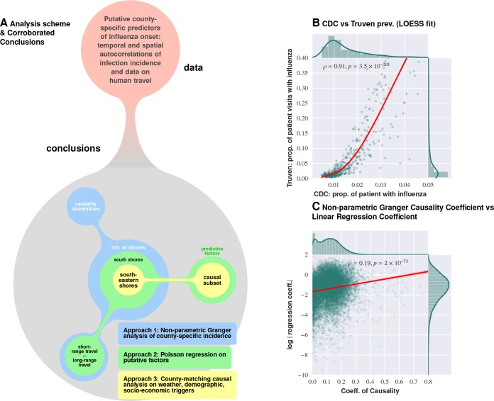
Figure 1—figure supplement 1. Logical flow and cross-corroboration of conclusions.

Plate A: Diverse data sets processed via multiple techniques to reach convergent, and reinforcing, conclusions. Approach 1 (the Granger-causality analysis) shows that the epidemic tends to begin near water bodies, and that short-range travel is more influential compared to air travel for propagation. Approach 2 (Poisson regression) identifies significant predictive factors, suggesting that the epidemic begins near the southern shores of the US, and corroborates the result on short- vs. long-range travel. Approach 3 (county-matching) points to south eastern shores of the continental US as where the epidemic initiates, and identifies a validated subset of predictive factors. Plate B shows that influenza prevalence as reported by Truven dataset positively correlates with CDC reports. Plate C illustrates that our conclusions regarding a putatively causal influence between neighboring counties, inferred using different techniques (mixed-effect regression vs. non-parametric Granger-causality), match up positively. Pearson’s correlation tests shown in Plates B and C are performed under null hypothesis that there the two types of quantities (plotted along axes X and Y) are statistically independent ($H_0:\rho =0$).

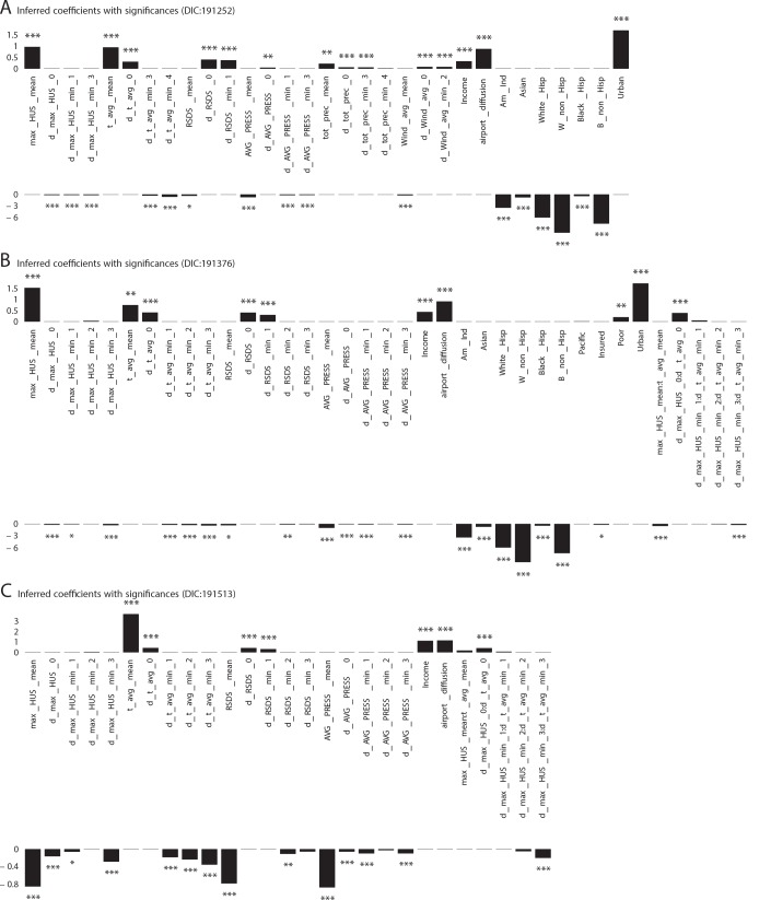
Figure 1—figure supplement 2. Significant influencing variables obtained with mixed effect regression with different models as tabulated in Table 1 of main text (three more models with DIC larger than that of the best model shown in Figure 1 plate A).

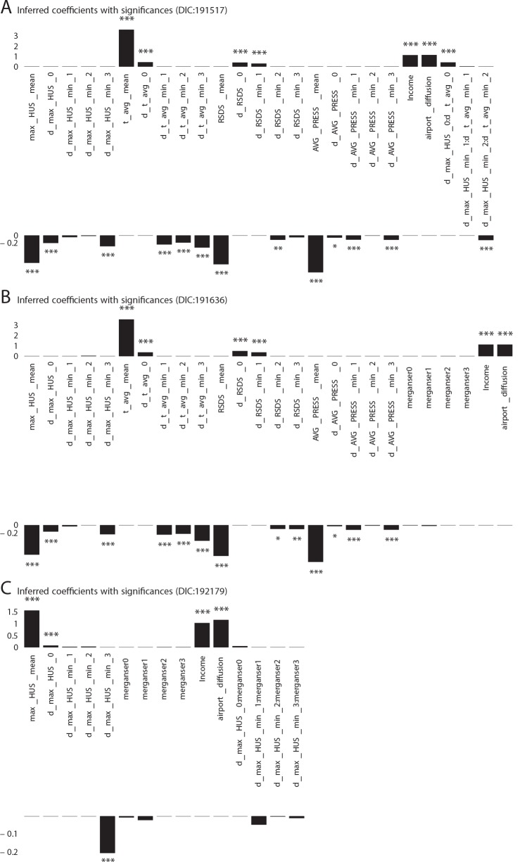
Figure 1—figure supplement 3. Additional Cases: Significant influencing variables obtained with mixed effect regression with different models as tabulated in Table 1 of main text (three more models with DIC larger than that of the best model shown in Figure 1 plate A).

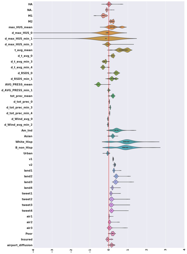
Figure 1—figure supplement 4. Violin plots for the coefficients inferred for variables that turn out to be significant in the best model, computed considering the complete set of models we investigated.

We note that with the exception of the antigenic variation of the surface protein hemagglutinin (HA), and some derivatives of maximum absolute humidity, significant mass of the individual violin plots fall either entirely on the positive or entirely on the negative half-plane; implying that the significant factors rarely flip sign. Thus, while the coefficients inferred change as we explore different models, the direction of influence remains mostly unchanged.

Figure 1—figure supplement 5. Spatial variation in the probability of patient visits corresponding to any ICD9-CM code (plate on left), and for diagnoses corresponding to influenza-like diseases (plate on right).

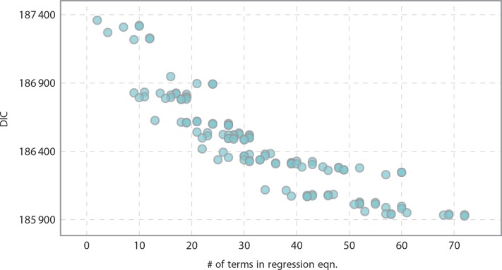
Figure 1—figure supplement 6. Informativeness of model vs model complexity as related to the number of terms in the regression equation.

As expected, we yielded more informative models as we increased complexity.