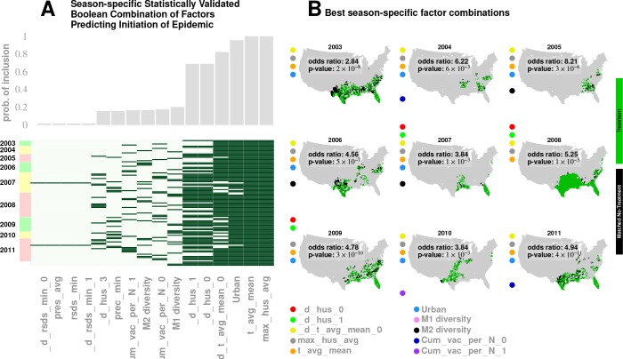
Figure 6. Results for our analysis involving county-matching (Approach 3).
Plate A illustrates the factor combinations that turn out to be significant over the nine seasons. Notably, for each season, we have multiple, distinct factor sets that turn out to be significant () and yield a greater-than-unity odd ratio. Plotting the probability with which different factors are selected when we look at season-specific county matchings (the top panel in Plate A), we see a corroboration of the conclusions drawn in Approach 2. We find that specific humidity and average temperature, along with their variations, are almost always included. We do see some new factors that fail to be significant in the regression analysis, , degree of urbanity and vaccination coverage. While vaccination coverage is indeed included as a factor in our best performing model, in Approach two it failed to achieve significance, perhaps due to its strong dependence on antigenic variation (see Figure 1J–M). Degree of urbanity is indeed significant for some of the regression models we considered (see Supplementary Information), but was not significant for the model with the smallest DIC. Note that ‘Treatment’ here is defined as a logical combination of weather factors. A treatment is typically a conjunction of several weather variables. For example, the treatment shown in top left panel of Plate B involves a conjunction of: (1) a drop in average temperature during the week of infection; (2) a drop in temperature during the week of infection; (3) a higher-than-average specific humidity; (4) a higher-than-average temperature, and; (5) a high degree of urbanity. With respect to the ‘treatment,’ we can divide counties into three groups: (1) ‘treated counties,’ shown in green; (2) at least one matching county for each of the treated counties (matching counties are very close to the treated counties in all aspects but in treatment, which we called ‘control’ counties), shown in black, and; (3) other counties, shown in grey. The counties in the ‘treatment’ and ‘control’ groups are further subdivided into those counties that initiated an influenza wave and those that have not, resulting in four counts arranged into a two-by-two contingency table. We then used the Fisher exact test to test for association between treatment and influenza onset. Panels in Plate B show both the treated and control sets for the seasons for a subset of chosen factors. The results are significant, as shown in Tables 2 and 3. The variable definitions are given in Table 4. Notably, some of the variables found significant in the regression analysis are not included above, and some which are not found to be significant in the best regression model show up here. This is not to imply that they are not predictive or lack causal influence. The matched treatment approach, as described above, is not very effective if we use more than factors simultaneously to define the treated set (for the amount of data we have); this results in a contingency table populated with zero entries.

