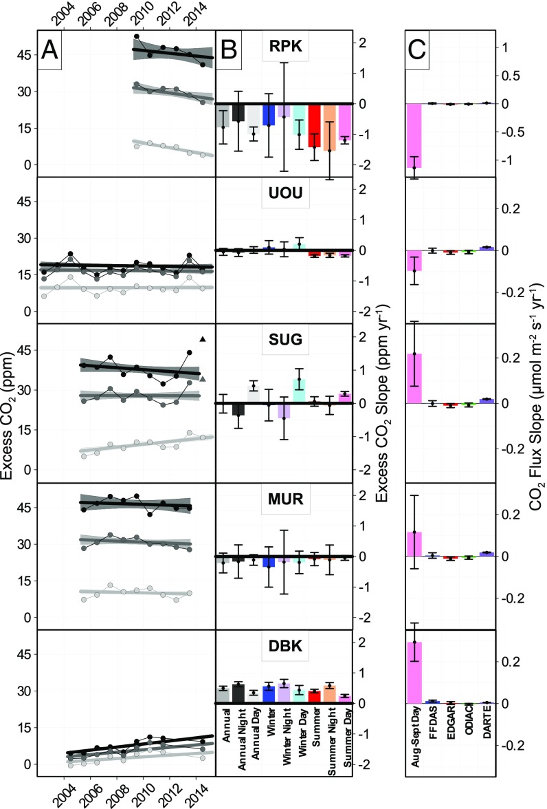
Fig. 3.

Time series and trends in SLV excess CO₂ mole fractions calculated from daily averaged data, with shading indicating ±2σ confidence intervals (A). Time series for the cold-season winter period (October–March), and the warm-season summer period (April–September) are shown in SI Appendix. Each panel contains three trends: the central trend using data from all hours of the day, the upper trend using nighttime data, and the lower trend using daytime data (hourly delineations: All hours: 00–23; Night: 00–05; Day: 12–17, LST). Symbols represent the average mole fractions from each year–season–time of day combination. The final year (2014) of observations at SUG were elevated due to an anomalous contribution from an apparent local source and were not included in the trends for that site (triangle symbol, SI Appendix). B shows the slope for each season and time of day trend, with 2σ confidence intervals (numeric values are listed in SI Appendix, Table S2). C shows the slope of the F_ff trends derived from observations averaged in August and September as well as from four fossil fuel inventories with 2σ confidence intervals. Note that the RPK panel has a different scale. See SI Appendix for flux calculation details and sensitivity tests.