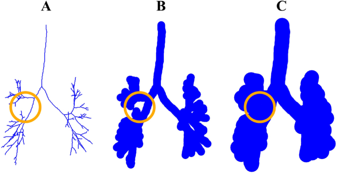
Figure 6.

Computing of branch-to-branch proximity. Consider the graph representing the bronchial tree as explained in Methods (A). This graph is called a tree since it contains no loops, i.e., no branches that bifurcate and then merge. Of note, there are many nodes (up to 264) between any two consecutive bifurcations, so the nodes appear dense in the graph representation. Centered at each node of this graph, we virtually set a ball of a fixed radius, thickening the construction. As we keep thickening more and more, by increasing the radius of those balls, at some point we will find that some branches merge, creating a loop (B). We record the radius r₁ at which this happens. For a large enough radius r₂, though, this loop will be filled in (C). If a merging of branches creates a loop that appears for the value r₁ of the radius and disappears at r₂, we represent this merging as the positive number r₂ − r₁. Summing up all these terms, we obtain a number we call branch-to-branch proximity.