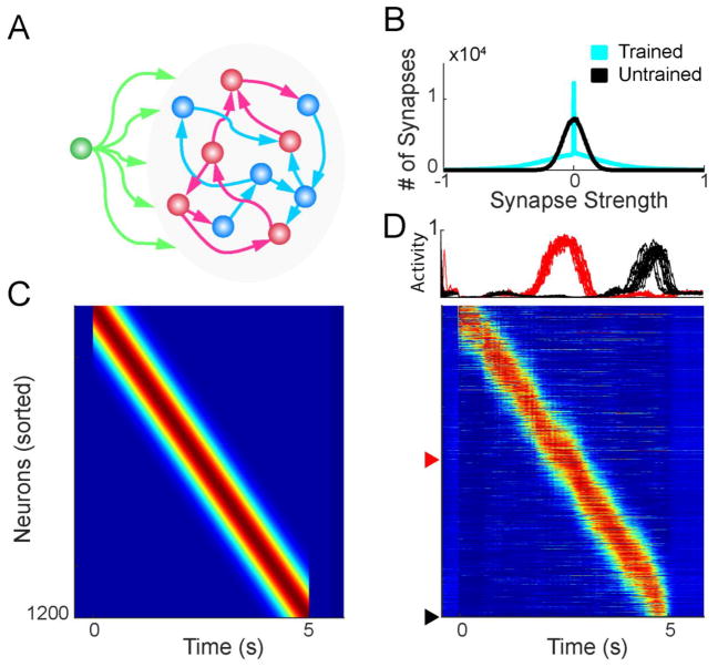
Figure 1. Generation of feedforward trajectories within a RNN.

A. Schematic of network architecture. The networks were composed of 600 excitatory (blue) and 600 inhibitory (red) firing rate units (N^Rec = 1200), with sparse recurrent connections. Neurons at the beginning of a sequence received input (green) during a 50 ms window to trigger the trajectory. B. Connection weights were initialized with a Gaussian distribution. After training to produce a single feedforward sequence, a large number of weights were pruned to zero, and some weights became stronger, resulting in a long tailed distribution. C. Example five second feedforward sequence target. D. After training, the RNN can produce a five second feedforward trajectory. Top: two units trained to activate in the middle and end of the trajectory, highlighted below. Each trace represents one of 15 trials. Bottom: Example network activity from a single trial.