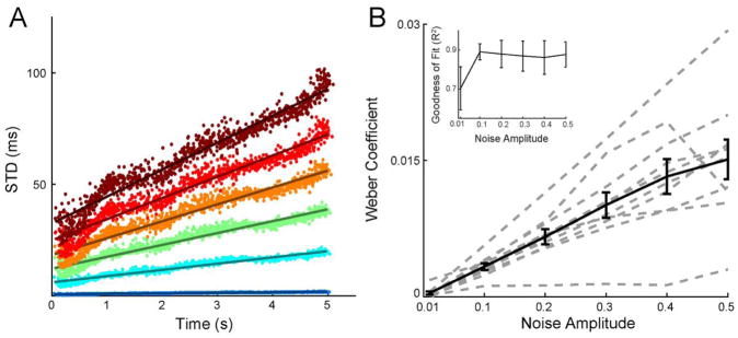
Figure 3. The timing generated by the RNN obeys Weber’s law.

A. Temporal variability increases linearly with elapsed time. Each dot shows the standard deviation of the activation time of a unit of an example network plotted against its mean. The activation time of each unit on each trial was determined from the center of a Gaussian fit of that unit’s activity. Each color represents one of six amplitudes of injected noise. Lines show the linear fit. B. The Weber law is robust to noise. The Weber Coefficient (slope of the linear fit shown in panel A) is shown across six noise amplitudes for ten trained networks. Each dotted line represent a single network, the solid black line represents the mean with error bars showing ± SEM. Inset: mean ± SEM of the goodness of fit (R²) for the linear fits.