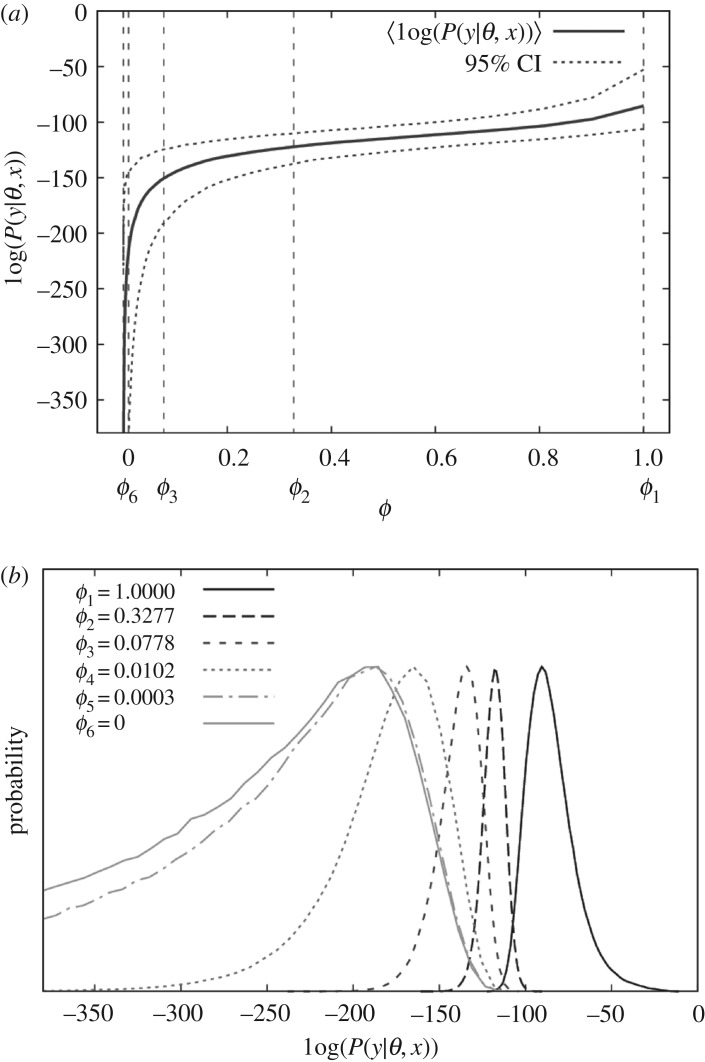
Figure 1.

(a) A typical example of how the posterior distribution in the log of the observed data likelihood varies as a function of inverse temperature ϕ. This distribution is represented by a mean (solid line) and 95% confidence intervals (denoted by the dotted lines). (b) The distributions for K = 6 chains from which samples are drawn during SS (with inverse temperatures defined by equation (2.4)).