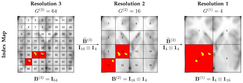
Fig. 1.

An example of multiresolution partitions and variable selection. Suppose a rectangle area in one axial slice cutting through brain that contains 64 regions (R = 64) is of interest. We consider three resolutions (K = 3). Three images in the right, middle, and left panels are labeled with the partition indices for the nested partitions at resolutions 3, 2 and 1 respectively. At the highest resolution (Resolution 3) there are 64 partitions (G⁽³⁾ = 64) with each partition including only one region and the partition indices are the same as the region indices, thus B⁽³⁾ = I₆₄. Resolution 2 has 16 partitions (G⁽²⁾ = 16) where each partition g contains four regions indexed by 4g − 3, 4g − 2, 4g − 1 and 4g, for g = 1, …, 16, indicating B̃⁽³⁾ = B⁽²⁾ = I₁₆ ⊗ 1₄, where ⊗ is Kronecker product. Resolution 1 has four partitions (G⁽¹⁾ = 4) where each partition g′ contains four finer-scale partitions at resolution 2 indexed by 4g′ − 3, 4g′ − 2, 4g′ − 1 and 4g′, for g′ = 1, …, 4, resulting in B̃⁽²⁾ = I₄ ⊗ 1₄; thus it contains 16 regions indexed by 16g′ − 15, 16g′ − 14, …, 16g′, for g′ = 1, …, 16, leading to B⁽¹⁾ = I₄ ⊗ 1₁₆. Suppose the true important voxels (yellow) are located in regions 39, 40 and 41. Valid posterior inferences for models at different resolutions produce high posterior inclusion probabilities of imaging biomarkers in the corresponding partitions (red) at all resolutions.