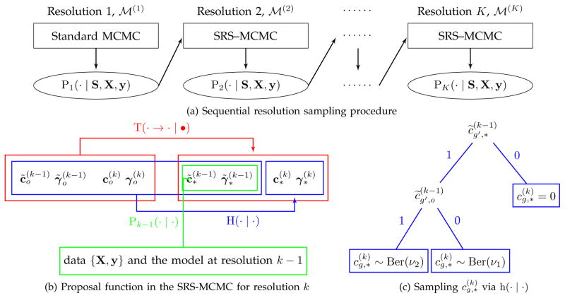
Fig. 2.
Illustration of sequential resolution sampling. (a) Initially, we utilize the standard MCMC algorithm to produce the posterior distribution of the selection indicators in
 at resolution 1, i.e. P1(· | S, X, y), which is then used to guide the construction of the proposal function in the SRS-MCMC algorithm to produce P2(· | S, X, y) for
 at resolution 2. This procedure is performed sequentially until resolution K to generate the posterior distribution PK(· | S, X, y) for our target model
 . (b) Decomposition of the proposal function T(· → · | •) (red) includes two steps for drawing a proposed sample. Step 1 (green): draw {
} from the posterior distribution Pk−1(· | ·) under the model
 at resolution k−1. Step 2 (blue): sample {
} given {
} in step 1 and the current state of the Markov chain using H(· | ·). (c) A binary tree represents the sampling scheme for
based on the probability mass function h(· | ·). It is determined by
and
for g′ satisfying
, and
.

