Decision-variable correlation

Abstract

An extension of the signal-detection theory framework is described and demonstrated for two-alternative identification tasks. The extended framework assumes that the subject and an arbitrary model (or two subjects, or the same subject on two occasions) are performing the same task with the same stimuli, and that on each trial they both compute values of a decision variable. Thus, their joint performance is described by six fundamental quantities: two levels of intrinsic discriminability (d′), two values of decision criterion, and two decision-variable correlations (DVCs), one for each of the two categories of stimuli. The framework should be widely applicable for testing models and characterizing individual differences in behavioral and neurophysiological studies of perception and cognition. We demonstrate the framework for the well-known task of detecting a Gaussian target in white noise. We find that (a) subjects' DVCs are approximately equal to the square root of their efficiency relative to ideal (in agreement with the prediction of a popular class of models), (b) between-subjects and within-subject (double-pass) DVCs increase with target contrast and are greater for target-present than target-absent trials (rejecting many models), (c) model parameters can be estimated by maximizing DVCs between the model and subject, (d) a model with a center–surround template and a specific (modest) level of position uncertainty predicts the trial-by-trial performance of subjects as well as (or better than) presenting the same stimulus again to the subjects (i.e., the double-pass DVCs), and (e) models of trial-by-trial performance should not include a representation of internal noise.

Extended signal-detection theory framework

The workhorse behavioral paradigm in many areas of human and animal research (e.g., perception, memory, decision making) is the two-alternative identification task. On each trial of an experiment, the subject is presented with a stimulus drawn from one of two categories, a and b, and is required to identify the category. The category identified by the subject (the subject's response) can be represented with capital letters A and B. Thus, on each trial there are four possibilities: The subject responds B when the category is b (B|b), the subject responds B when the category is a (B|a), the subject responds A when the category is a (A|a), or the subject responds A when the category is b (A|b). We note that the common two-alternative forced-choice task can be regarded as a special case where category a is a pair of stimuli in one spatial or temporal order and category b is a pair of stimuli in the opposite order.

Signal-detection theory (SDT) is the standard theoretical framework for interpreting the data measured in the two-alternative identification task (e.g., Green & Swets, 1974; Wickens, 2001). The theory assumes that the end result of all the processing in the organism, prior to the behavioral response, can be represented with a single, probabilistic decision variable that is described by one normal distribution if the stimulus is from category b and another normal distribution if the stimulus is from category a. The behavioral response is assumed to be generated by comparing the value of the decision variable on the trial to a criterion placed along the decision-variable axis. The subject makes one response if the value falls below the criterion and makes the other response if it falls above the criterion. In Bayesian statistical models, this decision variable would typically correspond to the log likelihood ratio—the log of the ratio of the probability of the modeled pattern of neural activity given category b to the probability given category a. However, it is important to point out that basic SDT makes no assumption about how the decision variable is computed. Its purpose is only to provide a principled interpretation of the four possible outcomes of trials in the identification task. Indeed, basic SDT can provide a principled interpretation even if there is no location within the nervous system where a single decision variable is represented.

Within the SDT framework, the probabilities of the four possible stimulus–response outcomes are determined by two parameters: the number d′ of standard deviations separating the two distributions, and the decision criterion . Thus, without loss of generality, the two normal distributions can be represented as normal distributions with standard deviations of 1.0 and means at and (Figure 1). In SDT, the parameter represents the intrinsic discriminability of the two categories, independent of the particular decision criterion adopted by the subject.

Figure 1.

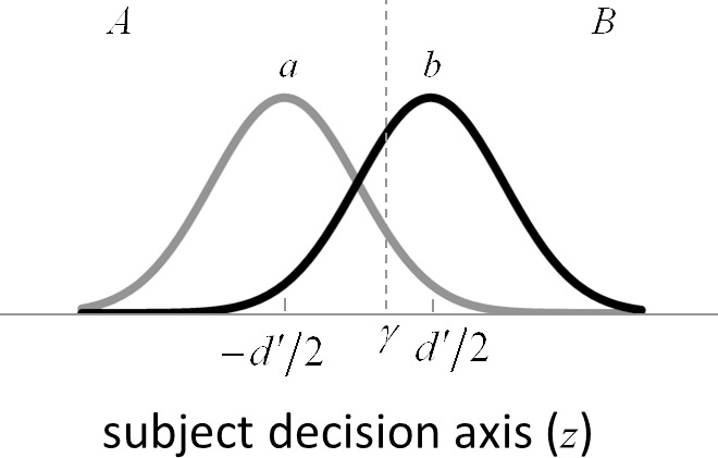
Standard signal-detection theory framework for interpreting responses in a two-alternative identification task. The two categories are represented by a and b, and the two possible behavioral responses by A and B. The discriminability of the two categories () is the number of standard deviations separating the distributions of the decision-variable values for the two categories. If the decision variable on a trial exceeds the decision criterion (), the response is B (the stimulus was from category b); otherwise the response is A.

A typical use of SDT is to estimate the subject's discriminability and decision criterion from the proportions of trials falling into the four possible stimulus–response outcomes already mentioned. Because the two proportions for each category must sum to 1.0, estimates of discriminability and criterion are obtained from just two proportions—for example, p(B|b) and p(B|a). In the special case of a yes–no detection task these two proportions represent the proportion of hits and false alarms (Green & Swets, 1974). These two proportions correspond to the areas under the two normal distributions above the decision criterion.

The estimates of the discriminability and the criterion are obtained by solving the following pair of equations:

where is the standard normal integral function. Two subjects could differ in their intrinsic ability to identify the categories (the values of ), in their decision biases (the values of ), or in both. SDT provides a principled framework for measuring these quantities, allowing better comparison of performance across subjects or between subjects and models.

The main goal here is to describe an extension of the standard SDT framework that allows measurement of two additional quantities (two decision-variable correlations) that provide increased power for comparing subjects and testing models. This is a straightforward extension related to existing signal-detection analyses, including the estimation of classification images (Ahumada & Lovell, 1971; Ahumada, 1996; for a review, see Murray, 2011), estimation of the ratio of external to internal noise (Spiegel & Green, 1981; Burgess & Colborne, 1988), and estimation of choice probabilities in neurophysiology experiments (Britten, Newsome, Shadlen, Celebrini, & Movshon, 1996; Haefner, Gerwinn, Macke, & Bethge, 2013; Pitkow, Liu, Angelaki, DeAngelis, & Pouget, 2015; Michelson, Pillow, & Seidemann, 2017; Seidemann & Geisler, in press).

Importantly, the extension proposed here does not require any special or new experimental design features; it can be applied to data from almost any two-alternative identification experiment in which the stimuli within each of the two categories are not physically identical on each trial. The only requirement is that the specific category and stimulus presented on each trial be known. There are many published studies where the experimenters saved the specific stimuli, or the information necessary to generate the stimuli (e.g., random-number seeds); however, there are also many studies where that is not the case. Another goal of this report is to emphasize the value of saving the stimuli, or the information for regenerating them, and the value of making the specific stimuli and responses publicly available.

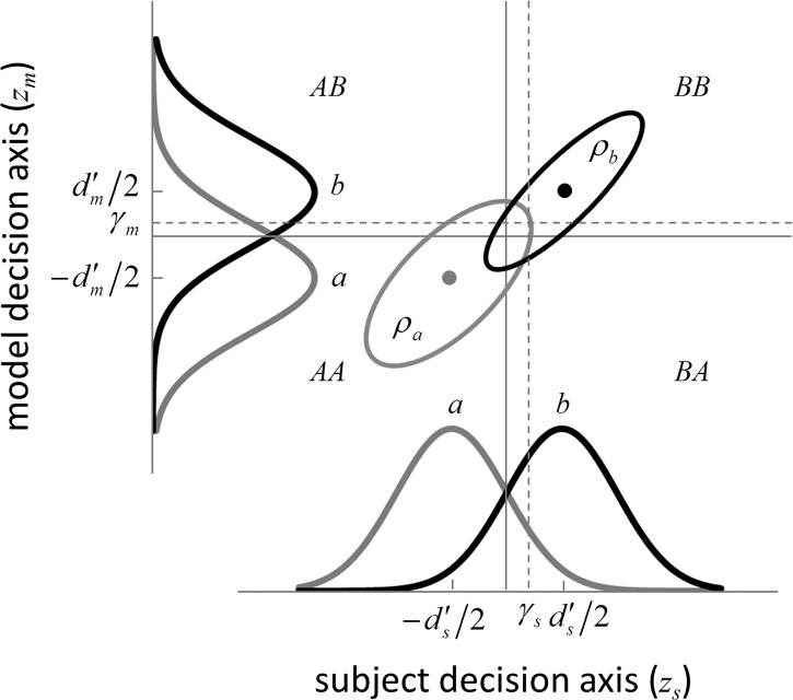
The extended SDT framework is illustrated in Figure 2. We assume that a subject and an arbitrary model (or two subjects, or the same subject on two occasions) are performing the same task with the same stimuli. Thus, we can represent the subject's normalized decision variable along the horizontal axis and the model's (or the second subject's) normalized decision variable along the vertical axis. The subject will have some arbitrary discriminability and some arbitrary decision criterion . Similarly, the model will have some arbitrary discriminability and some arbitrary decision criterion . As usual, Equations 1 and 2 can be used to estimate the discriminability and decision criterion of the subject and model from their respective response proportions , and , .

Figure 2.

Extended signal-detection theory framework for comparing subject (subscript s) and model (subscript m) performance in a two-alternative identification task. The horizontal axis represents the value of the subject's decision variable, and the vertical axis the value of the model's (or another subject's) decision variable. The Gaussians on each axis represent the distributions of the decision variable (normalized to a standard deviation of 1.0) for the two stimulus categories (a and b). The ellipses represent the joint (bivariate) distribution of the decision variables for the two stimulus categories. The bivariate distributions are completely described by four parameters: the d′ of the subject, the d′ of the model decoder, and the decision-variable correlations and . The four quadrants defined by the decision criteria (dashed lines) represent the different possible pairs of responses (first letter is the response of the subject, second is the response of the model).

An accurate model would have the same discriminability as the subject under the same conditions. However, even if a model has the same discriminability as the subject, the model and subject may vary in how correlated their responses are on a trial-by-trial basis. In the SDT framework, this is represented by the correlation between the decision variables. The better the model (or the more similar the two subjects), the higher is the correlation between the values of their decision variables (i.e., the more accurate the trial-by-trial predictions). These decision-variable correlations (DVCs) need not be the same for the two categories of stimuli. Thus, by measuring DVCs in addition to discriminabilities and decision criteria, we should have more power to discriminate between models, estimate model parameters, and characterize subjects based on individual differences.

The joint distribution of the two decision variables is given by one bivariate normal distribution for category a and another bivariate normal distribution for category b (represented by the ellipses in Figure 2). All the standard deviations are 1.0, because the decision variables are normalized. The mean for category a is at and for category b is at . The DVC for category a is and for category b is . Formally, the two distributions are given by

where is the standard bivariate normal density function

Once the discriminability and criterion values have been estimated from Equations 1 and 2, the DVCs can be estimated from four proportions that are directly available from the subject and model responses to the stimuli in each category. For category a they are the proportion of times the subject and the model both responded A, p(AA|a); the proportion of times the subject responded A and the model responded B, p(AB|a); the proportion of times the subject responded B and the model responded A, p(BA|a); and the proportion of times the subject and the model both responded B, p(BB|a). Similarly, for category b, the proportions are p(AA|b), p(AB|b), p(BA|b) and p(BB|b). These proportions correspond to the volume under the bivariate normal distribution within the four quadrants defined by the two decision criteria. As long as no more than one of the four proportions is zero, then it is straightforward to obtain the maximum-likelihood estimate of the DVC using Equations 3–5 (see Appendix). This estimate of the DVC is Pearson's tetrachoric correlation coefficient (Pearson, 1900; Stuart & Ord, 1991) applied in the SDT framework.

Maximum-likelihood estimation of the DVC from these four proportions is appropriate when only the categorical responses (A or B) are available, as when estimating DVCs between two subjects (or within the same subject on different occasions). However, for many (but not all) models, a decision variable is explicitly computed for each stimulus presentation. In this case, more reliable maximum-likelihood estimates can be obtained by directly using the values of the model's decision variable (see Appendix). However, we emphasize that DVCs can be measured even for a model that does not produce an explicit decision variable (e.g., some neural-network models).

The distributions of the decision variables for the subject and model (or another subject) are the marginal distributions of the bivariate distribution, and hence the DVCs do not necessarily depend on the discriminabilities and decision criteria estimated with basic SDT. The ellipses in Figure 2 represent a moderate positive correlation. If the decision variables were uncorrelated, then the ellipses would become circles. If the decision variables were negatively correlated, the ellipses would be rotated 90°. In principle, all of these correlations are possible for the same discriminabilities and decision criteria. For example, if a model and subject (or two subjects) are using different cues to perform a task, then it is possible that a stimulus that is easy for the model will be hard for the subject, and vice versa.

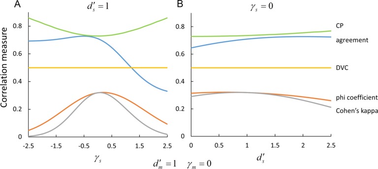
An important implication of this fact is that a given DVC can be consistent with many different values of standard measures of the behavioral correlation between the sequences of responses of the model and subject, or between two subjects. For example, Figure 3 shows how four different behavioral-correlation measures (defined in the Appendix) vary with the subject's decision criterion and discriminability , while the decision-variable correlation for category b is held fixed at 0.5 (yellow curves). The simplest correlation measure is the fraction of trials in which the subject and model are in agreement (blue curves). Perhaps the best-known and most common correlation measure for binary data is the phi correlation (also introduced by Pearson; Cramer, 1946, p. 282), which is equivalent to Matthews's (1975) correlation coefficient (orange curves). Another popular correlation measure is Cohen's (1960) kappa coefficient (gray curves). Finally, a common measure in the neurophysiology literature is choice probability (Britten et al., 1996; green curves). In all cases, the behavioral correlations vary substantially while the decision-variable correlation is held fixed. (We note that all the curves in Figure 3A are flipped about the vertical axis at 0 if the measures are computed for category a rather than category b.) In the extended SDT framework, the fundamental quantities are the discriminabilities, decision criteria, and DVCs. The overall accuracy levels and behavioral correlations depend in a rather complex way on all six of these fundamental quantities.

Figure 3.

Measures of behavioral correlation for a fixed value of the decision-variable correlation (yellow curves). The behavioral-correlation measures are the fraction of trials that the subject and model (or two subjects) make the same response to the same stimulus (blue curves); the phi coefficient, which is equivalent to the Matthews correlation coefficient (orange curves); Cohen's kappa coefficient (gray curves); and choice probability (green curves). (A) Value of behavioral-correlation measures as a function of the decision criterion, for a fixed discriminability of the subject. (B) Value of behavioral-correlation measures as a function of the subject's discriminability, for a fixed value of the decision criterion. Other than decision-variable correlation, most measures of the trial-by-trial relationship between a subject and model (or between two subjects) are rather strongly dependent on the values of the two decision criteria and discriminabilities. (The important thing to note here is the variation along the curves, not the vertical shifts between them.)

In other words, the extended SDT framework plays an analogous role in interpreting trial-by-trial correlations to the role that the standard SDT framework plays in interpreting accuracy. Standard SDT recognizes the fact that percent correct is not the best measure of accuracy because percent correct is dependent on the value of the decision criterion (every point on a given receiver operating characteristic curve corresponds to a different percent-correct value). Extended SDT recognizes the fact that previous trial-by-trial measures are not the best measures of trial-by-trial correlation because they are dependent on the value of decision criterion and the discriminability.

Simulations

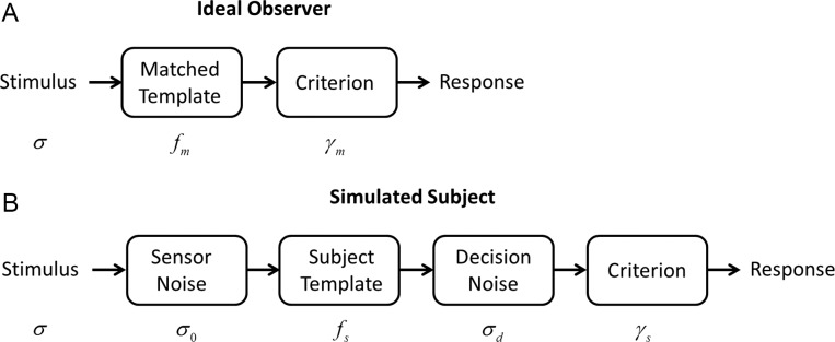
To better understand the implications of the SDT framework in Figure 2, we simulated model and subject decisions in the well-known task of detecting a target in white pixel noise. On each simulated trial we presented (with equal probability) a background of Gaussian white noise, or a background of noise plus an added target (a small Gaussian), to the simulated subject and to the model. We took the model to be the template-matching observer, which is the ideal observer for this particular task (Peterson, Birdsall, & Fox, 1954; Green & Swets, 1974; Burgess, Wagner, Jennings, & Barlow, 1981). On each trial, this model observer takes the dot product of the image with a template having the shape of the target:

where is the matched template and is the input image (Figure 4A). The template response is the (unnormalized) decision variable, which will have a normal distribution with the same standard deviation for target-present and target-absent trials. The normalized decision variable (as in Figure 2) was obtained by subtracting half the mean of the target-present response and dividing by the standard deviation.

Figure 4.

Model observers. (A) The ideal observer for detection in white noise (with standard deviation ) computes a matched-template response and then compares the template response to a decision criterion. (B) The family of suboptimal observers considered here has three suboptimal components: additive sensor noise with standard deviation , an arbitrary template , and late decision noise .

The simulated subjects were degraded versions of the ideal template-matching observer (Figure 4B). Two kinds of degradation were simulated. One kind was suboptimal pooling, which was obtained by removing some fraction of the pixels at random from the matched template (i.e., setting them to zero). The other kind of degradation was some level of simulated sensor noise—Gaussian white noise of standard deviation added to the input image. In other words, the simulated subjects could have inefficiency due to early noise, suboptimal pooling (sampling inefficiency), or both (e.g., Burgess et al., 1981; Burgess, 1985, 1994; Eckstein, Ahumada, & Watson, 1997; Lu & Dosher, 1999; Pelli & Farell, 1999). Later, we also consider the effect of decision noise.

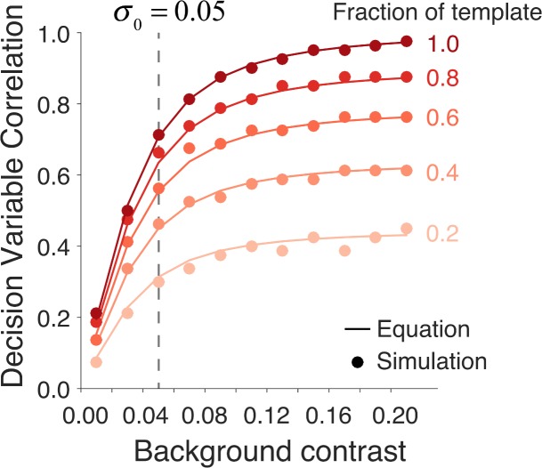
The symbols in Figure 5 plot the maximum-likelihood estimates of the DVC as a function of the root-mean-square (RMS) contrast of the background image (based on 500 trials per condition). These estimates were obtained from the categorical responses of the ideal observer and simulated subject (see Equations A1–A12). The solid curves show the expected DVC based on the closed-form expression derived in the Appendix (see Equation A33). Each curve is for a different fraction of remaining matched-template pixels. The RMS contrast of the neural noise was fixed at 0.05. The target amplitude was set so that the discriminability of the template-matching observer was 1.0 ().

Figure 5.

Decision-variable correlations between an ideal-observer model and a simulated subject in a two-alternative detection task. The horizontal axis is the root-mean-square contrast of a Gaussian white-noise background. Each curve is for a different simulated subject. All the simulated subjects had a fixed neural (pixel) noise corresponding to a root-mean-square contrast of 0.05. The simulated subjects differed in what fraction of pixels in the ideal observer's matched template they applied. The amplitude of the Gaussian target is set so that the discriminability of the ideal-observer model was fixed at 1.0. The solid curves show the functions expected from the closed-form expression (Equations A33–A36) derived in the Appendix.

DVC increases monotonically with background contrast. This is expected, because at low background contrasts the subject's decision variable is dominated by the neural noise. DVC also increases monotonically with the fraction of remaining pixels in the subject's template. This is also expected, because the subject's decision variable depends only on the background and neural variability at a subset of pixel locations. If the neural noise is set to 0.0, then all the curves in Figure 5 become horizontal lines. The DVCs in these simulations are the same for the two stimulus categories (here, target present and absent), but as mentioned before, this need not be the case in general. The simulations in Figure 5 demonstrate that DVC should vary systematically with fundamental properties of the subject and model, confirming that the extended SDT framework should be useful for testing models (and characterizing individual differences).

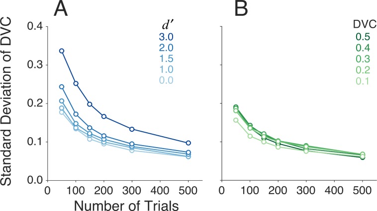
An obvious question is how the reliability of the estimate of DVC varies with the number of trials in the experiment, and with other aspects of the data. In any real situation, the confidence intervals could be estimated using bootstrap methods, but simulations are useful to get some idea of what to expect. Figure 6A plots the standard deviation of the estimated DVC as a function of the number of trials, for different levels of discriminability, when the true DVC was set to 0.5. These estimates were based on using only the categorical responses (see Appendix). The levels of discriminability were set by varying the amplitude of the target, with the neural and decision noise set to zero (Figure 4B). The DVC was set by removing pixels from the ideal matched template to obtain the simulated subject's template. (The relevant equations in the Appendix are A33–A38.) The results in Figure 6A make intuitive sense: As the level of discriminability goes up, there is less overlap of the distributions, and hence it takes more trials to reliably estimate the error proportions p(AB|b), p(BA|b), p(AB|a), and p(BA|a). For values of 2.0 or below, the estimates of DVC should be useful once the number of trials reaches about 100.

Figure 6.

Variability of decision-variable estimates based on simulations. (A) Standard deviation of decision-variable-correlation (DVC) estimates as a function of number of trials for a ground-truth DVC of 0.5, for several levels of discriminability. (B) Standard deviation of DVC estimates as a function of number of trials for a ground-truth value of 1.0, for several levels of DVC.

Figure 6B plots the standard deviation of the estimated DVC as a function of the number of trials, for different values of the true DVC, with the target amplitude set so that the discriminability () was fixed at 1.0. Interestingly, the standard deviation of the estimated DVC is not strongly dependent on the true correlation, at least over the range of 0.1 to 0.5 (the approximate range we observe in the demonstration experiment described later). In terms of percentage, the confidence interval shrinks nearly linearly with the true DVC.

Demonstration experiment

In addition to the simulations, we carried out and analyzed the data from a small experiment with two human subjects (the authors).

Methods

Psychometric functions were measured for detection of a Gaussian-shaped target having a standard-deviation parameter value of 4 arcmin, for three levels of Gaussian white-noise background contrast (0.05, 0.1, and 0.2 RMS) with a virtual pixel width of 2 arcmin (4 × 4 display pixels per virtual pixel) and mean luminance of 48 cd/m². The amplitude of the Gaussian target was defined to be the value at the peak of the target divided by twice the mean luminance (i.e., max amplitude = 1.0). The target and noise were presented for 250 ms in a blocked single-interval forced-choice task, with feedback. The three psychometric functions were measured three times for a total of 150 trials per target amplitude (total of 750 trials per psychometric function). The two subjects saw exactly the same stimuli, so that we could estimate between-subjects DVCs. In addition, we replicated the entire experiment with exactly the same trials a couple of weeks later (a double-pass experiment), so we could estimate within-subject DVC.

Results

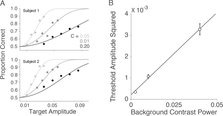
Figure 7A plots the measured psychometric functions for the two observers, for each level of background contrast. Figure 7B plots the estimated thresholds (the target amplitude when ). Consistent with previous studies (e.g., Burgess et al., 1981), the squared threshold amplitude increases linearly with background contrast power (the square of the RMS contrast).

Figure 7.

Psychometric functions and thresholds for background root-mean-square contrasts of 0.05, 0.1, and 0.2. (A) Psychometric functions for two subjects. (B) Average amplitude threshold squared as a function of background contrast power.

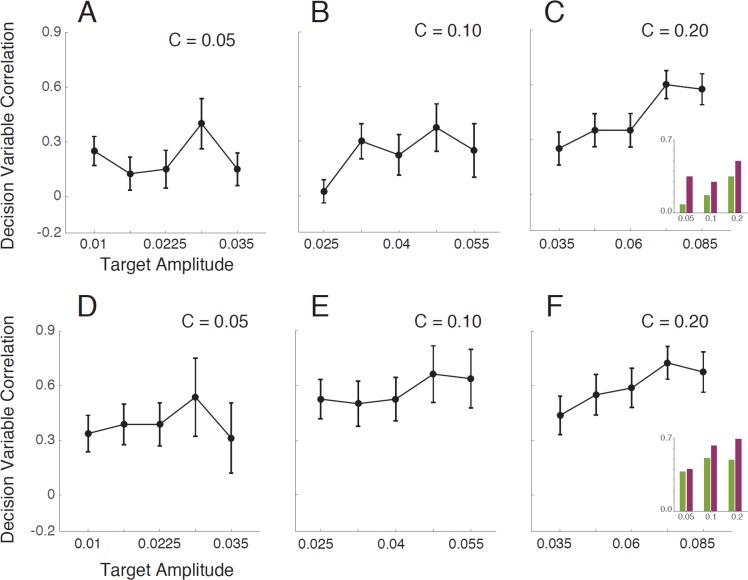
Figure 8A–8C plots the measured DVCs between the two subjects, as a function of target amplitude for each level of background contrast. Figure 8D–8F plots the measured within-subject (double-pass) DVCs. The DVC increases with background contrast; the average between-subjects correlations are 0.215, 0.258, and 0.425, and within-subject correlations are 0.398, 0.568, and 0.595. This result is qualitatively consistent with the hypothesis that the internal noise in the subjects is uncorrelated, and that as background contrast increases, the spatial structure of the external noise increasingly determines the values of the subjects' decision variables. The fact that the within-subject correlations are higher than the between-subjects correlations suggest that the templates (i.e., set of features) or internal noise levels of the two subjects are somewhat different.

Figure 8.

Between-subjects and within-subject decision-variable correlations (DVCs). (A–C) DVC between the two subjects as a function of target amplitude for the three levels of background root-mean-square contrast. (D–F) DVC of the subjects with themselves, based on the double-pass responses to the same stimuli. Shown here is the average of the two subjects. Error bars are bootstrapped 67% confidence intervals. The pattern is similar for the two subjects, although they differ somewhat in the magnitude of correlation; average DVC for S1 is 0.465; for S2, 0.575. The insets show the average DVCs at each background contrast for target-present (purple) and target-absent (green) trials.

Interestingly, there is a trend for the DVC to increase with target amplitude, especially when background contrast is high, and a trend for DVC to be greater for target-present than target-absent trials (see insets and schematic ellipses in Figure 2). This is not consistent with the family of model observers in Figure 4B, even though the model observers correctly predict that threshold energy should increase linearly with background energy (Figure 7B). Specifically, this family of models predicts that neither the contrast of the target nor its presence or absence should have an effect on the DVC. In simple simulations, we have found that these trends are predicted if the two subjects (or the same subject on two occasions) have different levels of intrinsic position uncertainty (a factor not included in Figure 4B; but see later).

In the Appendix we show that for the class of models in Figure 4B, the double-pass experiment provides an estimate of the correlation of the subject's template to that of the ideal matched template. Specifically, the cosine similarity between the subject's template and the ideal matched template equals the square root of the ratio of the subject's efficiency to the double-pass DVC:

where the efficiency is defined as . Furthermore, we show that if (in addition) the late decision noise is negligible compared to the sensor noise, then the double-pass DVC provides an estimate of the ratio of the sensor-noise standard deviation to that of the external stimulus noise:

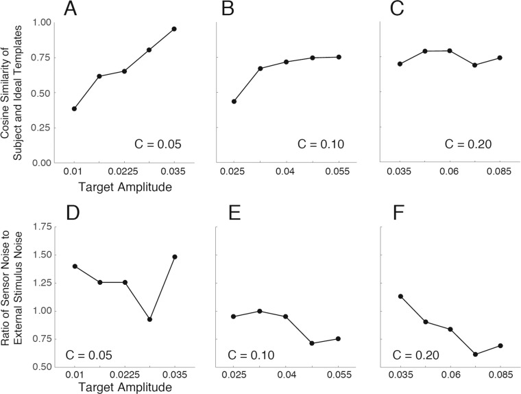
Figure 9A–9C plots the estimated correlations of the subjects' templates to the ideal template, and Figure 9D–9F plots the estimated relative standard deviation of the subjects' sensor noise (under the strong assumption that late decision noise is negligible). These plots illustrate how DVCs can provide constraints useful for estimating the components of multistage models like the one in Figure 4B.

Figure 9.

Template cosine similarity and internal- to external-noise ratio. (A–C) Estimated cosine similarity of the subjects' and ideal observer's templates (Equation 7) as a function of target amplitude, for the three background contrasts. (D–F) Estimate of the ratio of internal sensor-noise level to external noise level (Equation 8) as a function of target amplitude, for the three background contrasts.

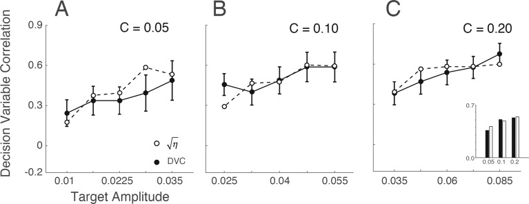
The solid circles in Figure 10A–10C are the DVCs between the template-matching ideal observer and the subjects, as a function of the target contrast. As expected, the DVCs are lower than those within the subjects. In the Appendix we show that the family of model human observers in Figure 4B predicts that the DVC between the human and ideal observers should equal the square root of the efficiency:

Figure 10.

Decision-variable correlation (DVC) between subjects and ideal observer as a function of target amplitude, for the three levels of background root-mean-square contrast. The solid symbols are the DVCs averaged across the two subjects. The error bars are bootstrapped 67% confidence intervals. The open symbols show the DVCs predicted from the subjects' efficiencies, for the family of models in Figure 4B. The inset shows, for each background contrast, the DVC (solid bars) and square root of efficiency (open bars) averaged across target amplitude.

The open symbols in Figure 10A–10C are the square-root of the efficiency. Remarkably, this prediction appears to hold quite well.

However, as in Figure 8 there is a trend for the DVC to increase with target amplitude. Thus, the pattern of results is not consistent with the class of models in Figure 4B, unless it is extended to allow the template, sensor noise, or decision noise to vary with target contrast.

The demonstration experiment and various formulas derived in the Appendix show that computing DVCs can provide considerable additional power for testing models of performance, beyond the power provided by computing only detectabilities (i.e., psychometric functions and thresholds) and decision biases.

Estimating model parameters

A strong model will not only predict the accuracy of the subjects in each condition but will also predict the trial-by-trial responses—the more accurate the prediction of the trial-by-trial responses in a condition, the larger the DVC. The best specific model in a parameterized family of models can be found by finding the parameters that maximize the predicted accuracy and DVC. The most efficient procedure for doing this will likely depend on the family of models and the specific task the subjects are performing.

As an example, consider the present detection-in-noise task and the family of models in Figure 4B, generalized to include the possibility of position uncertainty. This family of models assumes that the subject applies a template on each trial and compares the responses of that template to a decision criterion. Note that in this section we regard Figure 4B as the model observer (not the simulated subject), and thus its responses, criterion, template, and detectability will have the subscript m.

DVCs can be exploited to estimate the subject's template and level of position uncertainty. Using classification-image techniques (Ahumada, 1996; Murray, 2011), Eckstein, Beutter, Pham, Shimozaki, and Stone (2007) found that subjects' templates for detecting Gaussian targets in noise have approximately the shape of a difference-of-Gaussians function. Thus, here we assumed that the model observer's template is a difference-of-Gaussians function with three parameters, two standard deviations and a relative weight for center and surround: (the center is scaled by and the surround by ). The model observer in Figure 4B does not take into account the effects of position uncertainty, which is likely to be an important factor (Solomon, 2002; Tjan & Nandy, 2006). Thus, we generalized the model observer to allow inclusion of position uncertainty. Specifically, the template is now applied over a spatial region with a radius of pixels, and the model observer's unnormalized decision variable is the maximum of these template responses:

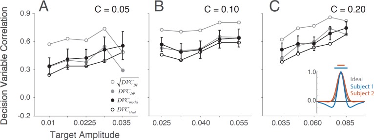
To estimate the subjects' template and level of uncertainty, we set the model observer's sensor and decision noise to zero (i.e., the response to a given stimulus is deterministic) and varied the difference-of-Gaussians parameters and the uncertainty parameter to maximize the average DVC of the model observer and subjects.

The inset in Figure 11 shows the estimated templates and uncertainty regions for the two subjects; the estimated model parameters are given in the figure caption. The solid black circles in the panels show DVCs between the model observer and subjects. For comparison, the open black circles show the DVCs between the ideal observer and subjects from Figure 10, and the solid gray circles show the double-pass DVCs from Figure 8D–8F. Remarkably, the model observer is able to predict the trial-by-trial responses of the subjects as accurately as, or more accurately than, presenting the same stimulus again to the subjects. This is possible because the model observer does not have sensor or decision noise, whereas, the subject has independent samples of sensor and decision noise on both trials with the same stimulus. In the Appendix (Equation A51), we show that the upper limit for DVC, given the model observers in Figure 4B, is the square root of the double-pass DVC (open gray circles in Figure 11).

Figure 11.

Decision-variable correlation (DVC) of a model observer. The solid black circles show the DVC (with the subjects) of a model observer having a difference-of-Gaussians template and a circular spatial-uncertainty region. The open black circles show the DVC of the ideal observer from Figure 10. The solid gray circles show the double-pass DVC of the subjects from Figure 8. The open gray circles show upper limit of possible DVC for model observers. As in earlier figures, the plots show the average DVC for the two subjects; however, the model-observer parameters were estimated separately for each subject. The inset shows the ideal template and the templates for the two subjects (normalized to a peak of 1.0); the horizontal lines show the diameter of the estimated uncertainty region. Model parameters for S1: , , , . Model parameters for S2: , , , .

This example demonstrates the potential usefulness of DVCs for estimating model parameters. It also demonstrates the important principle that, in general, models that optimally predict an organism's trial-by-trial responses should not include a representation of neural noise within the organism. Thus, there is a fundamental difference between predicting trial-by-trial responses and predicting other aspects of performance (e.g., neural noise is needed to explain why the subjects' double-pass DVCs are not 1.0). This principle also holds for models of neural response—in general, an optimal model of trial-by-trial neural responses will be deterministic and will predict the responses better than presenting the same stimuli twice.

Discussion

Experiments measuring behavioral performance in humans and other animals often use a task where the stimulus on each trial is drawn from one of two categories, and the subject is required to identify the category. Such tasks are particularly common in the areas of perception, memory, and decision making. In all of these areas, the well-known framework of signal-detection theory (SDT) is commonly used to estimate both the subject's intrinsic ability to identify the category () and the subject's decision bias (). We described a straightforward extension of SDT that can provide additional power for testing models and quantifying individual differences. Responses to the same stimuli are recorded from a model and a subject, from two subjects, or from the same subject on two occasions. From these responses, six quantities are estimated (see Figure 2): two discriminability (identifiability) values, two decision-criterion values, and two decision-variable correlations (DVCs; one for each stimulus category). The discriminability and decision-criterion values are estimated in the usual way (e.g., from hits and false alarms). The DVCs can be estimated from the pairs of categorical responses to the stimuli within each category, or (for many models) from the subject's categorical responses and the model's continuous decision-variable values.

DVC is a principled measure of the relationship between the trial-by-trial responses made by a subject and a model, two subjects, or the same subject on multiple occasions. We found that other common measures of correlation in trial-by-trial behavior do not properly take into account the effects of discriminability and decision bias on the estimation of correlation (see Figure 3). We then demonstrated and evaluated the extended framework in simulations and in an experiment involving detection of a Gaussian-shaped target in Gaussian white noise. Even this very simple experiment yielded a rich set of theoretical and experimental results. We found that it was possible to derive a new set of predicted relations for the well-known class of models in Figure 4. These relations allowed us to reject this class of models for detection in white noise. We then estimated parameters for an extended model and found that it is possible to predict trial-by-trial performance as well as or better than presenting the same stimuli twice to the subject. Finally, we showed that deterministic models are best for predicting trial-by-trial performance, while models with sources of internal noise are necessary to explain other aspects of performance.

Measuring DVCs

Estimation of DVCs requires that, in a given condition (e.g., a specific background contrast and target amplitude), the two categories contain multiple stimuli (exemplars). In many published studies, a given condition consists of exactly the same two stimuli presented multiple times (e.g., discrimination experiments with fixed stimuli). In these cases, all of the trial-to-trial variation in the subjects' responses is due to unknown internal factors (e.g., neural noise). Because these experiments vary the stimuli so little, they provide less information for testing hypotheses about the underlying neural computations (and neural noise). In general, we argue it is much better (and more realistic compared to real-world tasks) to include some stimulus variation within conditions.

To compute DVCs between two subjects, it is necessary to present the same stimuli to both subjects. This is easy to do and is potentially useful for characterizing individual differences in trial-by-trial behavior. For example, if a number of subjects are tested on the same stimuli, then those with similar neural processing should have higher DVCs.

To compute DVCs on the same subject, it is necessary to present the same stimuli (at least) twice to the same subject (a double-pass experiment). As we saw, double-pass experiments can also be very useful within the context of a specific class of models. In addition, they can provide a useful benchmark. For many models, the maximum possible DVC between the model and subject is the square root of the DVC between subject and herself. However, a double-pass experiment is a special design that, it could be argued, is inefficient because it doubles the length of the experiment.

In contrast, computing DVCs between a subject and a model requires nothing more than keeping track of the specific stimuli and responses on each trial of the experiment. For stimuli that are randomly generated or sampled this can be as simple as describing the random-number generator, saving the random-number seed, and saving a short sequence of random numbers (this makes it possible to verify later that the random-number generator is behaving as expected and hence that the regenerated stimuli are correct). Even if an experimenter is not immediately interested in trial-by-trial behavior, saving this information and making it available would make it possible for others to compute DVCs or other measures of the trial-by-trial performance.

Computing DVCs between subjects and models is useful for testing models. In principle, all six quantities in the extended SDT framework can be estimated for every stimulus condition in an experiment. For example, in the small experiment described here there were 15 conditions (5 target amplitudes × 3 background contrasts). The 90 estimated quantities (d′s, criteria, and DVCs) provide a strong set of constraints on models of detection in white noise. Of course, in some experimental designs there may not be sufficient trials to reliably estimate all six quantities for each condition. Even so, estimates can be averaged across conditions and can still be useful for testing hypotheses. For example, in the demonstration experiment, computing the average DVC (across the five target amplitudes) for each of the three background contrasts would have been sufficient to provide a strong test of the model in Figure 4B—the average correlations approximately equal the square root of the average efficiencies.

The extended SDT framework is most directly applied in experiments with blocked conditions, where a number of responses are collected for each pair of fixed stimulus categories. For experiments where the categories are continuously varying (e.g., adaptive psychophysical procedures) it should still be possible to apply the framework by binning the stimuli into approximately fixed categories.

Robustness to violations of the equal-variance assumption

The extended SDT framework makes the standard SDT assumption that the decision variables for the two categories, in a given condition, are normally distributed with equal variance (Figures 1 and 2). This assumption is likely to hold only approximately. We carried out calculations to get some idea about how robust the estimated quantities are to the violations of this assumption. Specifically, we varied the ratio of the variances of the two normal distributions. We set and , where k is the ratio of the two variances, with the sum of the variances equal to 2.0 (i.e., the average variance is 1.0). We set , , and the criterion at the cross point between the distributions. We assumed this is true for both the subject and model (or both subjects). For a true DVC of 0.5 (which was the same for both categories) we first computed the proportion of responses in the four quadrants for each category (see Figure 2) and then estimated assuming equal variances. Figure 12 shows how the estimated discriminability, criterion, and DVC varied as a function of k (e.g., k = 0.5 to 2). As the ratio of the variances deviates from 1.0 there are modest systematic deviations of the estimated discriminability and criterion from the actual values. Interestingly, there is no systematic error in the estimate of the DVC. Overall, the extended SDT framework appears to be fairly robust to violations of the equal-variance assumption.

Figure 12.

Robustness of extended signal-detection theory framework to violation of the equal-variance assumption. The solid curves show the estimated values of , , and (see Figure 2) as function of the ratio of the variances of decision variable for the two categories a and b. The values of the estimated discriminabilities, criteria, and decision correlations are the same for both the subject and model, because the means, variances, and correlations of the decision variables were set to be the same in the calculations. The dashed curves show the actual values.

Relationship between DVC, choice probability, and choice correlation

Choice probability (CP) and choice correlation (CC) are popular measures of the trial-by-trial relationship between measured neural responses and behavioral responses (Britten et al., 1996; Haefner et al., 2013; Pitkow et al., 2015). CP and CC are typically computed only in neurophysiological studies, but they could potentially be computed when evaluating the trial-by-trial predictions of a behavioral model. Specifically, one could regard the value of a model's decision variable on a trial as a hypothetical neural response. CP is defined to be the probability of correctly discriminating the subject's behavioral responses, given the neural responses, using the standard SDT framework. In the Appendix we derive the formal relationship between DVC and CP. CC is an approximately linear function of CP, and is equivalent to computing a DVC computed under certain assumptions. Under these assumptions there is a one-to-one relationship between the measures, but like the other measures of trial-by-trial correlations, CP and CC are dependent on the subject's discriminability and decision criterion (see Figure 3). Thus, DVC is a more general and flexible measure for evaluating models and should also be better for evaluating the relationship between neural activity and behavior (see also Michelson et al., 2017; Seidemann & Geisler, in press).

Appendix

Maximum-likelihood estimation of decision-variable correlation (DVC): Categorical responses

Here we consider maximum-likelihood estimation of the DVC when all the available responses are categorical. This is appropriate when computing DVCs between two subjects, the same subject on different occasions, or a model and a subject when the model does not generate a continuous decision variable on each trial (e.g., some kinds of neural-network models).

In the extended SDT framework, the proportion of trials in the four quadrants defined by the two decision criteria correspond to the volume under the bivariate normal distribution in those quadrants. Given Equations 3 and 5, the four integrals for category b are

and for category a they are

The log likelihood of the data given the DVC for category b is

and for category a it is

where are the proportions of observations in the four quadrants for category b and are the proportions of observations in the four quadrants for category a. The maximum-likelihood estimates of the two DVCs are obtained by finding the maxima of the log likelihoods given by Equations A9 and A10:

For those who use MATLAB we note that

with , , , and .

Similarly,

with , , , and .

Inspection of Figure 2 shows that if at least three of the four quadrants contain a nonzero proportion of trials, then some constraints are placed on the possible DVC. However, if there are just two nonzero proportions, then the DVC is essentially unconstrained. This happens when one or more of the decision criteria does not sufficiently overlap the joint distribution. One case where this can happen is if the subject's accuracy is too high. Another case is if the subject is highly biased. For example, if the subject makes no false alarms, then the DVC cannot be measured for the target-present category (although it may still be measurable for the target-absent category). In general, to estimate at least one of the DVCs, both the model and the subject (or the two subjects) must make some errors.

Note that the proportions in the four quadrants defined by the decision criteria must sum to 1.0 for each category. Thus, there are a total of six independent measured quantities, which exactly matches the number of parameters to estimate (2 d′ values + 2 decision criteria + 2 DVCs).

Maximum-likelihood estimation of DVC: Model decision-variable responses

Here we consider maximum-likelihood estimation of the DVC when the continuous value of the decision variable of the model observer is available (e.g., when the decision variable is the log likelihood ratio of the two categories given the stimulus). This is the preferred method to estimate DVCs when the model decision variable is available, because it is generally a more reliable estimate (notice smaller error bars in Figures 10 and 12 than in Figure 8).

Let be the categorical (binary) response of the subject on trial i, and let be the value of the model observer's normalized decision variable on trial i (i.e., its value in the space of Figure 2). For category a, the log likelihood of all the subject's responses given the value of the model's decision variable is given by

where

with

Note that is the standard normal integral function (in MATLAB, ). The maximum-likelihood estimate of the DVC is found by maximizing Equation A15 over all possible values of the DVC:

We now derive Equation A17. From the definition of conditional probability (and Figure 2), we have

where is the standard bivariate normal density function (Equation 5) and is the standard univariate normal density function, where , , and . From Equations 5 and A19 we have

Completing the square in the exponent and simplifying gives

Substituting for y and x_c gives Equation A17.

Equations analogous to A15 to A18 hold for estimating the DVC for category b. The main difference is that

Finally, note that when the values of the model decision variable are available, then DVCs can be estimated as long as the subject makes some errors (no errors need be made by the model).

DVC between optimal and suboptimal observers

In the simulations, the stimulus on target-present trials is

and on target-absent trials it is

where is white Gaussian noise with a variance of and is the mean luminance. The target shape is defined to have a maximum of 1.0. The amplitude of the target is a. We simulated and analyzed two kinds of observers: the ideal template-matching observer and suboptimal model subjects (see Figure 4).

The ideal observer's matched template is defined to be the target shape normalized by its energy,

where represents the dot-product operator defined in Equation 6. Thus, the unnormalized decision-variable value on target-present trials is

and on target-absent trials it is

The model subject's template is an arbitrary template, and we assume that the simulated subject has some additive independent neural noise with variance and some late decision noise with variance (see Figure 4). Thus, the simulated subject's unnormalized decision-variable value on target-present trials is given by

and on target-absent trials it is given by

The correlation between the decision variables is

The covariance and standard deviations are unaffected by additive constants (the target and mean background luminance), and thus the DVC (in the present case) is the same for both categories of trials (target present and target absent):

From the definition of covariance and standard deviation, we have

Thus,

where is the cosine similarity of the subject and model templates,

is the ratio of the internal-noise variance to the external-noise variance,

and is the ratio of the decision-noise variance to the external-noise variance scaled by 1 over the subject template energy,

We also note that

and

Therefore, the efficiency of the simulated subject is

Dividing top and bottom by yields

and so

Thus, this simulated subject satisfies the strong constraints that the DVCs be the same for both stimulus categories, and the DVC equals the square root of the efficiency (compare Equations A33 and A42):

In other words, for this class of subject models the DVC with the ideal observer is completely determined by the discriminabilities. Note that this relation holds for every specific background and target contrast. Thus, it holds for the more general class of models where the neural noise, subject template, and decision noise vary as a function of background and target contrast.

DVC between the same suboptimal observers

A useful technique for estimating the relative effect of internal and external noise on an observer's performance is the double-pass technique, where the subject is presented the same stimuli twice during the experiment (Swets, Shipley, McKey, & Green, 1959; Spiegel & Green, 1981; Burgess & Colborne, 1988). The data from double-pass experiments can also be analyzed by estimating the DVC of the subject with herself in the two passes. For the class of model human observers considered here, the first- and second-pass responses are given by

In other words, the sample of external noise is the same, but the samples of neural noise and decision noise are different. The DVC in the double-pass experiment is

Thus, for this class of subject model, the double-pass decision correlation provides an estimate of :

If one assumes that there is no late decision noise, then the double-pass decision correlation provides an estimate of , the ratio of the internal-noise to external-noise variance (see also Burgess & Colborne, 1988).

Comparison of Equations A42 and A47 shows that

Thus, the data from the double-pass experiment also provide an estimate of the cosine similarity of the subject and model template,

However, the double-pass experiment does not provide an estimate of the relative contributions of early neural noise and late decision noise.

If the subject is using the optimal template (or the same template as a model observer; i.e., ), and has only neural and decision noise, then Equations A33 and A47 imply that

Behavioral-correlation measures

Here we define the three behavioral-correlation measures plotted in Figure 3.

The fraction of trials where responses are in agreement is given by

The phi coefficient (Matthew's correlation coefficient) is given by

Cohen's kappa coefficient is given by

where and

Relationship between DVC and choice probability (CP)

CP is the probability of correctly discriminating the subject's behavioral responses, given the value of a model's decision variable, using the standard SDT framework. In neurophysiology experiments this decision variable is computed from the neural responses on a trial, and in the present case it is computed from the stimulus on a trial. In the notation of Figure 2, CP can be computed for each stimulus category. For category a the two relevant distributions are and . For category b they are and . CP is then usually defined as the area under the receiver operating characteristic (ROC) for the pair of distributions. Equivalently, one can compute the choice probability from the hits and false alarms for the optimally placed criterion. Consider trials for category a. From Bayes's rule we have

Using Equations A17 and 2, and the fact that , we have

The proportions of hits and false alarms are given by

Finally, the CP in the current single-interval task is given by

Figure A1.

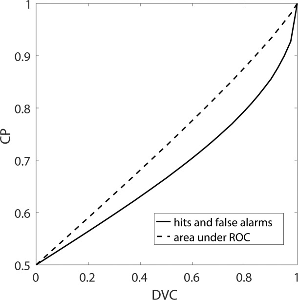
Relationship between equivalent choice probability (CP) and decision-variable correlation. Equivalent CP is defined to be the CP when the subject's criterion is located at the peak of the subject's decision-variable distribution. The solid curve gives the equivalent CP as a function of the decision-variable correlation for single stimulus presentations—the probability of correctly identifying the response the subject made, given the value of the model's decision variable. The dashed curve gives the CP that would be obtained for two stimulus presentations: one where the subject responded A, and one where the subject responded B. In this case, the curve gives the probability of correctly identifying on which of the two presentations the subject responded B given the two values of the model's decision variable (this corresponds to the area under the receiver operating characteristic curve). The area under the receiver operating characteristic curve is standard, but is a bit inflated because it is not the actual trial-by-trial accuracy of predicting the subject's choices (solid curve).

The area under the ROC in a single-interval task actually gives the percent correct that would have occurred in a two-interval task. This slightly inflated accuracy is obtained by dividing by rather than in Equation A60.

Analogous equations hold for category b:

The values of CP depend on the subject's discriminability and decision criterion, and on the DVC, but not on the model's discriminability; thus, these equations can be simplified by setting . If there is a desire to express the DVC as an equivalent CP, then one method is to estimate the DVC as described here, substitute the value into these equations, and then set the subject's criterion to align with the peak of the subject's decision-variable distribution, which has the same effect as setting and . Figure A1 shows the relationship between CP and DVC when and , based on hits and false alarms, and based on the area under the ROC.

References

- Ahumada, A. J.,, Jr. (1996). Perceptual classification images from Vernier acuity masked by noise [Abstract]. Perception, 25 Suppl. 1, 2, https://doi.org/10.1068/v96l0501. [Google Scholar]
- Ahumada, A. J.,, Jr.,, Lovell, J. (1971). Stimulus features in signal detection. The Journal of the Acoustical Society of America, 49, 1751– 1756. [Google Scholar]
- Britten, K. H., Newsome, W. T., Shadlen, M. N., Celebrini, S., Movshon, J. A.. (1996). A relationship between behavioral choice and the visual responses of neurons in macaque MT. Visual Neuroscience, 13, 87– 100. [DOI] [PubMed] [Google Scholar]
- Burgess, A. E. (1985). Visual signal detection: III. On Bayesian use of prior knowledge and cross correlation. Journal of the Optical Society of America A, 2, 1498– 1507. [DOI] [PubMed] [Google Scholar]
- Burgess, A. E. (1994). Statistically defined backgrounds: Performance of a modified non-pre-whitening matched filter model. Journal of the Optical Society of America A, 11, 1237– 1242. [DOI] [PubMed] [Google Scholar]
- Burgess, A. E., Colborne, B.. (1988). Visual signal detection: IV. Observer inconsistency. Journal of the Optical Society of America A, 5, 617– 627. [DOI] [PubMed] [Google Scholar]
- Burgess, A. E., Wagner, R. F., Jennings, R. J., Barlow, H. B.. (1981, October 2) Efficiency of human signal discrimination. Science, 214, 93– 94. [DOI] [PubMed] [Google Scholar]
- Cohen, J. (1960). A coefficient of agreement for nominal scales. Educational and Psychological Measurement, 20 1, 37– 46, https://doi.org/10.1177/001316446002000104. [Google Scholar]
- Cramer, H. (1946). Mathematical methods of statistics. Princeton, NJ: Princeton University Press. [Google Scholar]
- Eckstein, M. P., Ahumada, A. J., Watson, A. B.. (1997). Visual signal detection in structured backgrounds: II. Effects of contrast gain control, background variations, and white noise, Journal of the Optical Society of America A, 14, 2406– 2419. [DOI] [PubMed] [Google Scholar]
- Eckstein, M. P., Beutter, B. R., Pham, B. T., Shimozaki, S. S., Stone, L. S.. (2007). Similar neural representations of the target for saccades and perception during search. The Journal of Neuroscience, 27, 1266– 1270. [DOI] [PMC free article] [PubMed] [Google Scholar]
- Green, D. M., Swets, J. A.. (1974). Signal detection theory and psychophysics. Huntington, NY: R. E. Krieger Publishing; (Original work published 1966 by John Wiley & Sons, Inc.). [Google Scholar]
- Haefner, R. M., Gerwinn, S., Macke, J. H., Bethge, M.. (2013). Inferring decoding strategies from choice probabilities in the presence of correlated variability. Nature Neuroscience, 16, 235– 242. [DOI] [PubMed] [Google Scholar]
- Lu, Z. L., Dosher, B. A.. (1999). Characterizing human perceptual inefficiencies with equivalent internal noise. Journal of the Optical Society of America A, 16, 764– 778. [DOI] [PubMed] [Google Scholar]
- Matthews, B. W. (1975). Comparison of the predicted and observed secondary structure of T4 phage lysozyme. Biochimica et Biophysica Acta—Protein Structure, 405 2, 442– 451, https://doi.org/10.1016/0005-2795(75)90109-9. [DOI] [PubMed] [Google Scholar]
- Michelson, C. A., Pillow, J. W., Seidemann, E.. (2017). Majority of choice-related variability in perceptual decisions is present in early sensory cortex. bioRxiv, 207357, https://doi.org/10.1101/207357.
- Murray, R. F. (2011). Classification images: A review. Journal of Vision, 11 5: 2, 1– 25, https://doi.org/10.1167/11.5.2. [DOI] [PubMed] [Google Scholar]
- Pearson, K. (1900). Mathematical contributions to the theory of evolution—VII: On the correlation of characters not quantitatively measurable. Philosophical Transactions of the Royal Society of London, Series A, 195, 1– 47. [Google Scholar]
- Pelli, D. G., Farell, B.. (1999). Why use noise? Journal of the Optical Society of America A, 16, 647– 653. [DOI] [PubMed] [Google Scholar]
- Peterson, W. W., Birdsall, T. G., Fox, W. C.. (1954). The theory of signal detectability. Trans. IRE PGIT, 4, 171– 212. [Google Scholar]
- Pitkow, X., Liu, S., Angelaki, D. E., DeAngelis, G. C., Pouget, A.. (2015). How can single neurons predict behavior? Neuron, 87, 411– 423. [DOI] [PMC free article] [PubMed] [Google Scholar]
- Seidemann, E., Geisler, W. S.. (in press). Linking V1 activity to behavior. Annual Review of Vision. [DOI] [PMC free article] [PubMed]
- Solomon, J. A. (2002). Noise reveals visual mechanisms of detection and discrimination. Journal of Vision, 2 1: 7, 105– 120, https://doi.org/10.1167/2.1.7. [DOI] [PubMed] [Google Scholar]
- Spiegel, M. F., Green, D. M.. (1981). Two procedures for estimating internal noise. The Journal of the Acoustical Society of America, 70, 69– 73. [DOI] [PubMed] [Google Scholar]
- Stuart, A., Ord, J. K.. (1991). Kendall's advanced theory of statistics, Vol. 2. New York, NY: Oxford University Press. [Google Scholar]
- Swets, J. A., Shipley, E. F., McKey, M. J., Green, D. M.. (1959). Multiple observations of signals in noise. The Journal of the Acoustical Society of America, 31, 514– 521. [Google Scholar]
- Tjan, B. S., Nandy, A. S.. (2006). Classification images with uncertainty. Journal of Vision, 6 4: 8, 387– 413, https://doi.org/10.1167/6.4.8. [DOI] [PMC free article] [PubMed] [Google Scholar]
- Wickens, T. D. (2001). Elementary signal detection theory. Oxford, UK: Oxford University Press. [Google Scholar]