Algorithm for rapid determination of optical scattering parameters

Abstract

Preliminary experiments at the NIST Spectral Tri-function Automated Reference Reflectometer (STARR) facility have been conducted with the goal of providing the diffuse optical properties of a solid reference standard with optical properties similar to human skin. Here, we describe an algorithm for determining the best-fit parameters and the statistical uncertainty associated with the measurement. The objective function is determined from the profile log likelihood, including both experimental and Monte Carlo uncertainties. Initially, the log likelihood is determined over a large parameter search box using a relatively small number of Monte Carlo samples such as 2·10⁴. The search area is iteratively reduced to include the 99.9999% confidence region, while doubling the number of samples at each iteration until the experimental uncertainty dominates over the Monte Carlo uncertainty. Typically this occurs by 1.28·10⁶ samples. The log likelihood is then fit to determine a 95% confidence ellipse.

The inverse problem requires the values of the log likelihood on many points. Our implementation uses importance sampling to calculate these points on a grid in an efficient manner. Ultimately, the time-to-solution is approximately six times the cost of a Monte Carlo simulation of the radiation transport problem for a single set of parameters with the largest number of photons required. The results are found to be 64 times faster than our implementation of Particle Swarm Optimization.

1. Introduction

The measurement of the scattering parameters of optical tissue phantoms has been underway since the late twentieth century. [1–3] Optical scattering for biological tissues has been reviewed recently. [4, 5] Various measurements techniques, in the time domain, [6, 7], in the frequency domain, [8, 9] in the spatial domain using either fiber-based [10, 11] or non-contact [12, 13] techniques, and using one or two integrating spheres, [14–18] were used to measured the optical properties of liquid and solid phantoms.

In the past decade, the need for optical tissue phantoms which mimic the properties of human skin has been a prominent issue. After polytetrafluoroethylene (PTFE) was found to have attenuation parameters far from human skin, [19] other reference phantoms were sought, including both solid [20] and liquid [21, 22] samples. Liquid phantoms mixing Intralipid, [23] a lipid solution of calibrated scatterers and India Ink as an absorber have been proposed as a reliable reference sample with accurate values of the reduced scattering coefficient ${\mu }_s^{\prime }$ and the absorption coefficient μ_a [7, 10, 24] and were used for inter-comparison studies. [25] Intralipid is more economical than calibrated polystyrene micro-spheres and hence is more practical for the production of large batches of liquid phantoms. However, solid phantoms are preferred since they are easier to disseminate and tend to be more stable in time. They typically use a base material such as polyurethane or polydimethylsiloxane (PDMS) with an added mixture of titanium dioxide (TiO₂) powder or aluminum oxide (Al₂O₃) powder to match the desired scattering coefficient and an absorber such as India Ink, carbon black, carbon nanotubes, or 9096 dye to match the desired absorption coefficients. [20, 26, 27] Other materials such as polyvinyl chloride plastisol (PVCP) have been used for phantoms. [28]

As part of the National Institute of Standards and Technology’s (NIST) current effort to develop a reference measurement service for the optical properties of biomedical phantoms, [29] in this study we present measurements of solid biomedical phantoms manufactured by the Institut National d’Optique (INO, Quebec, Canada) using NIST’s Spectral Tri-function Automated Reference Reflectometer (STARR) goniometric instrument for measuring angle resolved scattering (ARS) functions in reflectance and transmittance. An inversion algorithm based on a Monte Carlo model is used to estimate the optical scattering parameters μ_a and μ_s and confidence regions from the measured ARS.

This paper focuses on the inversion algorithm including its time-to-solution and its ability to estimate the statistical uncertainty of the measurement. Issues of validity of the measurement and intercomparisons with other national metrological institutes will be the subject of future communications.

Recently, a algorithm based on Particle Swarm Optimization (PSO) for determining diffuse optical parameters in a different measurement geometry was presented. [30] Because of that work and the fact that PSO is a very widely used method today, [31] we implement PSO for comparison.

2. Measurements

2.1. Samples and physical measurements

The phantoms are polyurethane-based with added carbon black and TiO₂ to match the nominal values of μ_a and ${\mu }_s^{\prime }$ at a wavelength specified below. The phantoms are square slabs with a nominal lateral dimension of 100 mm and present a specular face resulting from the surface tension while molding and a rough face resulting from machining to obtain a specified thickness. The phantoms were prepared from one batch of material, INO B0455, with nominal thicknesses of 6 mm, 8 mm and 10 mm and a nominal μ_a = 0.01 mm⁻¹ and ${\mu }_s^{\prime }=1{\text{ mm}}^{-1}$ at λ = 800 nm. The actual thicknesses of the samples were measured with a dial gauge micrometer at nine locations on a 3×3 grid with a center point set near the center of the sample. The variance of the measured thickness $s_d^2$ was combined with the uncertainty attributable the precision of the dial micrometer $u_{\text{dial}}^2$ to compute the combined uncertainty associated with thickness, $u_d^2=s_d^2+u_{\text{dial}}^2$. In this paper we use coverage factor k = 2, unless noted. The measured thickness values t are 6.10±0.09 mm, 8.10±0.11 mm, and 10.12±0.06 mm. These values are used in the simulation.

2.2. Index of refraction

A bench-top spectrophotometer equipped with an integrating sphere detector (Lambda 1050, Perkin-Elmer, Waltham, MA, USA) was used to measure the Fresnel reflectance from the specular face of the sample at an 8° incident angle by subtracting the diffuse reflectance measured with the specular port of the sphere open from the total diffuse reflectance measured with the specular port blocked (measurements corrected from the background signal). The Fresnel reflectance was measured from λ = 400 nm to λ = 1000 nm in steps of 10 nm and using the Fresnel equation for unpolarized light at 8° incident angle, the index of refraction n of the sample bulk material was obtained. Measuring the composite material with Fresnel reflectance is consistent with the definition of the index of refraction in MCML. The values were fit to the Cauchy dispersion law between 450 nm and 850 nm yielding values for the index at λ = 543 nm, 632 nm, and 805 nm. The results are n₈₀₅ = 1.493 ± 0.010, n₆₃₂ = 1.498 ± 0.011, and n₅₄₃ = 1.502 ± 0.012. In arriving at these uncertainty estimates, the standard deviation was found among four measurements of the three samples (the 6 mm sample having been measured twice).

2.3. Angle-resolved scattering

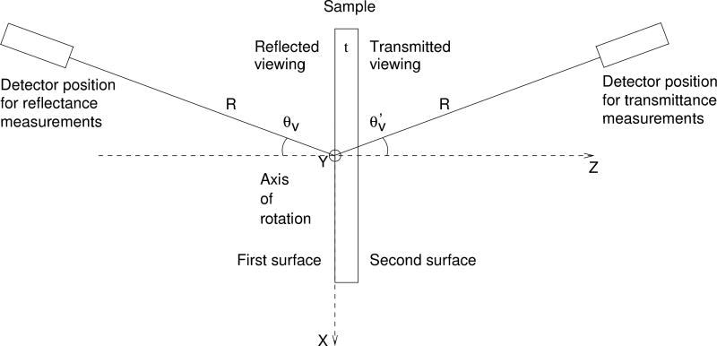
Measurements of the angle-resolved scattering (ARS) functions were performed using NIST’s STARR, [32] a home-built instrument which serves as the national reference for spectral bidirectional reflectance measurements. The instrument also allows measurement of spectral bidirectional transmittance measurements. Measurements provided by STARR are absolute. Validation measurements were made prior to the experiments using a check standard composed of sintered polytetrafluoroethylene (PTFE). The results were found to be in the tolerance range. A schematic is shown in Fig. 1. Each sample was measured at three different wavelengths, λ = 543 nm, 632 nm, and 805 nm, at a polarization state either parallel or perpendicular to the plane of incidence. The measurements were averaged over polarization.

Fig. 1.

Experimental schematic for the ARS measurements. Here, R is distance between the sample first face and the detector aperture θ_ν is the viewing angle in reflectance, ${\theta }_{\nu }^{\prime }$ is the viewing angle in transmittance, and t is the thickness of the sample.

The radiant flux from the source (a quartz-tungsten-halogen lamp) is focused through an order-sorting filter and a shutter onto the entrance slit of a single-grating monochromator. The beam exits the monochromator and is collimated by an off-axis parabolic mirror. It then passes through a Glan-Taylor polarizer before passing through the sample goniometer. The beam is collected by the detector aperture, and is focused by a lens onto the detector (ultraviolet-enhanced silicon photodiode), which produces a signal proportional to the radiant flux. The translation and rotation stages of the goniometer enable the acquisition of both reflected or transmitted and incident signals. The sample is positioned in the holder so that it is normal to the incident beam. The detector rotates around the sample to collect the reflected or transmitted signals at various viewing angles, which are in the same plane as the sample normal and the incident beam. The incident radiant flux is measured by positioning the detector in the incident light beam with the sample translated out of the beam.

The viewing angles, θ_ν in reflectance and ${\theta }_{\nu }^{\prime }$ in transmittance, are about the axis of rotation which is the vertical axis Y. Below, we will report the transmittance angle by extending θ_ν to cover the range 0° to 180°, using ${\theta }_{\nu }=\pi -{\theta }_{\nu }^{\prime }$. The data was collected with θ_ν incremented from 5° to 180° in 5° steps, excluding θ_ν = 90°.

The first surface of the sample coincides with the vertical plane defined by the X and Y axes. The distance between the first surface of the sample and the detector aperture is R = 669.8 mm. The aperture has an area A = 796.7 mm². The ARS is

$$\mathit{\text{ARS}}=\frac{P_s}{\mathrm{\Omega }{P}_i}$$ (1)

where P_i is the incident power measured by the detector when no sample is present and P_s is the power scattered from the area of the sample included in the detector field of view at angles within the solid angle defined by Ω = A/R². This formula applies in both transmission and reflectance.

3. Theory

Although we are concerned with the measurement of particular scattering parameters, the general question of estimating parameters from experimental data is an inverse problem. In a typical inverse problem, there is a physical theory (known in engineering as a “forward model”) which gives predictions based on values of some input parameters. One varies the parameters to achieve a best fit under some criterion such as least-squares. Said differently, the parameters are chosen to maximize some objective function.

We follow this paradigm with a wrinkle: our predictions are based on a Monte-Carlo algorithm so the predictions come with an uncertainty which can be reduced for a price: additional Monte Carlo trials. With sufficient trials, we can approximate the exact predictions of the theory to any specified accuracy. However, the use of Monte Carlo to calculate optical properties has been considered to be impractical due to excessive computation time, [2, 10, 18, 33] although Monte Carlo methods have been used to determine the optical properties of tissues in the context of the double integrating sphere [34] and a homogeneous semi-infinite medium. [35] Other methods used to solve the inverse problem in optical scattering include Alerstam et al. [36] who use scaling methods, Chen et al. [37] who vary the parameters and keep random numbers constant to send photons on similar trajectories, and Kholodtsova et al. [30] who use Particle Swarm Optimization (PSO).

We take advantage of the following circumstances: (a) the fits tend to get worse as the parameters become farther removed from their optimum values and (b) very bad parameters can be eliminated from consideration with relatively few Monte Carlo trials. Schematically, we will sample a few values from the full allowed search space for the parameters with a relatively small number of Monte Carlo trials. From the quality of the fits, we obtain a somewhat smaller search region. We increase the Monte Carlo trials and iterate the procedure. At some point, the experimental uncertainties are much greater than the Monte Carlo uncertainties and the iterations can stop. In the present case, we found 7 or 8 iterations were sufficient. The process is highly efficient: if we double the number of Monte Carlo trials at each stage, then half of the trials will be taken in the final stage because ${\sum }_{n=0}^{N-1}{2}^n\approx 2^N$.

We obtain an additional acceleration by using importance sampling to find our objective function, a profile log likelihood as explained below, on a grid of points for three times computational cost than obtaining the log likelihood for a single pair of parameters. Further computational speed is obtained by using a parallel random number generator SPRNG. [38, 39]

3.1. The forward model: radiation transport with Monte Carlo

For our forward model, we re-implemented the MCML [40] code in C++. MCML is the de facto standard in the field of biomedical optics: the original paper has been cited over 1800 times according to Web of Science. MCML is a computer program for Monte Carlo modeling of light transport in multilayer tissues. The material is assumed to be infinite in the x y plane and consists of a finite number of layers with surfaces orthogonal to the z axis. In our case, there is a single layer. Each layer is characterized by the following optical parameters: the index of refraction n, the absorption coefficient μ_a, the scattering coefficient μ_s, and the anisotropy factor g. For reference, g is the parameter in the Henyey-Greenstein scattering function [41]

$$p_{\mathit{\text{HG}}}(\theta ;g)=\frac{1-g^2}{2{(1+g^2-2g\text{ cos }\theta )}^{3/2}},$$ (2)

where θ is the scattering angle and p_HG(θ) is a probability distribution. We often compute using the transformed variables μ_t = μ_a + μ_s and η_a = μ_a/μ_t.

We rely on an earlier determination of the scattering anisotropy factor g = 0.621 ± 0.015 (k = 1) at 660 nm, measured in the single scattering regime. [20] We neglect dispersion in the anisotropy factor. We find that varying g and μ_s such that ${\mu }_s^{\prime }={\mu }_s(1-g)$ is constant leads to no discernible change when g is varied between 0.521 and 0.721 which is a k = 6.7 expanded uncertainty.

The program models the light particles as being unpolarized and incoherent. When photons encounter boundaries, whether internal or external, they are transmitted or reflected according to the Fresnel reflectance and transmittance formulas. Absorption is modeled through deweighting the particle for the absorption in the layer it is traveling through. Scattering is modeled through Monte Carlo sampling. Refraction according to Snell’s law is also included.

In MCML, particles leaving either the front or back surface are scored according to their direction of travel. In our implementation, after exit, we trace particles into annular bins located at a finite radius which represent the detector. If the photon is traveling through air in the direction ν̂ from position r⃗₀ inside a circle of radius R, its line of travel is described by

$$\overrightarrow{r}=\alpha \hat{\nu }+{\overrightarrow{r}}_0$$ (3)

where α is the directed distance. The intersection of the line in Eq. (3) with a circle of radius R occurs at

$$\alpha =-{\hat{\nu }}_0·{\overrightarrow{r}}_0+{[{({\hat{\nu }}_0·{\overrightarrow{r}}_0)}^2+R^2-r_0^2]}^{1/2}$$ (4)

which is positive for R > r₀. Physically, this is true because the sample is smaller than the distance to the detector. Eq. (3) and Eq. (4) together give the point on the detector; an annular bin can be found through the arc tangent function.

3.2. The objective function: profile log likelihood

Because we are interested in both best-fit values (called “point-estimates” in the field of statistics) and confidence regions, we employ a likelihood-based algorithm. We assume that the uncertainty in each measurement is unknown, but equal. This allows us to handle the nuisance parameters associated with measurement uncertainty and Monte Carlo error using the profile log likelihood. [42] We prefer the ARS to the bidirectional reflectance and transmittance distribution (BRDF and BTDF) functions, which provide equivalent information, because the ARS comes closer to obeying the equal uncertainty condition.

Our likelihood model is given somewhat abstractly next. Let y_i be the measurements, indexed from i = 1 to N. In our case, these are the reflectance or transmittance measurements at a given angle. Let Θ be a list of parameters of length ν to vary (such as μ_a and μ_s, leading to ν = 2, with fixed parameters such as the thickness t, the index of refraction n, and the anisotropy scattering parameter g implicit) and let α̂_i (Θ; N_phot) be a particular prediction from the Monte Carlo code. For the i^th measurement using N_phot photons. The Strong Law of Large Numbers applies here so that α̂_i (Θ; N_phot) converges to a constant, α_i (Θ), as N_phot grows large. We model this process as

$$y_i={\alpha }_i(\mathrm{\Theta })+{\epsilon }_i$$

$${\hat{\alpha }}_i(\mathrm{\Theta })={\alpha }_i(\mathrm{\Theta })+{\delta }_i$$ (5)

where ε_i and δ_i are independent mean zero normal deviates with variance ${\sigma }_{\epsilon }^2$ and ${\sigma }_{\delta }^2$, respectively. Here, ε_i describes the measurement error and δ_i describes the Monte Carlo error.

The above implies that

$$y_i-{\hat{\alpha }}_i(\mathrm{\Theta })~\text{Normal}(0,{\sigma }_{\epsilon }^2+{\sigma }_{\delta }^2).$$ (6)

Letting the variance $V={\sigma }_{\epsilon }^2+{\sigma }_{\delta }^2$, the log likelihood is

$$\ell (\mathrm{\Theta },{\mu }_s^{\prime },V)=-\frac{N}{2}\text{log}(2\pi )-\frac{N}{2}\text{log}(V)-\frac{1}{2V}\sum _{i=1}^N{[y_i-{\hat{\alpha }}_i(\mathrm{\Theta })]}^2$$ (7)

using natural logarithms. Since V is a nuisance parameter, it is profiled (or optimized) out of the log likelihood. Taking the derivative with respect to V, setting the derivative to zero, and solving for V gives

$$V=\frac{1}{N}\sum _{i=1}^N{[y_i-{\hat{\alpha }}_i(\mathrm{\Theta })]}^2,$$ (8)

i.e., the mean square difference of the measurements and the Monte Carlo predictions. Plugging the optimized value for V back into ℓ gives

$${\ell }_P({\mu }_a,{\mu }_s^{\prime }=-\frac{N}{2}\{\text{log }\left[\frac{1}{N}\sum _{i=1}^N{[y_i-{\hat{\alpha }}_i(\mathrm{\Theta })]}^2\right]+\text{log}(2\pi )+1\}.$$ (9)

An approximate confidence region is obtained by finding all values of x⃗ such that

$${\ell }_P({\overrightarrow{x}}_{\mathit{\text{mle}}})-{\ell }_P(\overrightarrow{x})\le \frac{1}{2}{({\chi }_{\nu }^2)}^{-1}(p)$$ (10)

where ${({\chi }_{\nu }^2)}^{-1}(p)$ is the inverse of the χ² cumulative distribution function with ν degrees of freedom, and p is a confidence level such as 0.95 [43].

3.3. The optimization algorithm: iterative refinement guided by confidence regions

The profile log likelihood yields confidence regions that include contributions of uncertainty from both Monte Carlo and fixed errors (namely, measurement error and model mismatch). In a baseline algorithm, we would use a large number of Monte Carlo runs so that the uncertainty attributable to the fixed errors dominate. However, to do that across a large set of points in the (μ_a, μ_s) plane, requires a considerable amount of computation, as evidenced by its implementation on graphics processing units (GPUs). [44]

However, as discussed above, here we double the number of Monte Carlo samples at each iteration which will lower the Monte Carlo contribution to the uncertainty. Eq. (9) can be used to shrink the search region at each iteration.

In our implementation, we start with 2 · 10⁴ Monte Carlo samples and double this value at each iteration, typically to a maximum value of 1.28 · 10⁶. shrinking the search space each time. We shrink the search space by excluding any points outside of a 99.9999% confidence region. We also impose an ad hoc rule that the search space will never shrink by more than a factor of 2 at any given iteration. In practice, this rule comes into effect only in the first couple of iterations.

3.3.1. Importance Sampling

A major difference between the forward problem and the inverse problem is that we require the solution to the forward problem on a grid of points to perform the inverse problem. Here, we use importance sampling to produce predictions for a grid of points in our parameter space with one set of random numbers. Importance sampling dates back several decades, but its early use was as a variance reduction technique. [45] The idea has strong antecedents even in the field of optical scattering. Graaff et al. [35] varied the single-scattering albedo (1 − η_a in our notation) analytically to produce results for several values without rerunning the Monte Carlo simulation. Sassaroli et al. [46] extended the weighting procedure to scattering events. Hayakawa et al. [47, 48] used the technique in perturbative Monte Carlo (pMC) to values for alternative parameters as well as differential Monte Carlo (dMC) to produce derivative of objective functions. They implement the technique for inverse problems in one variable.

In our code, we follow the MCML code [40] in using the variables of (a) the inverse of the mean interaction length μ_t = μ_s + μ_a, where ${\mu }_s^{-1}$ is the mean scattering length and ${\mu }_a^{-1}$ is the mean absorption length and (b) the absorption fraction η_a = μ_a/μ_t. At each iteration, we specify a rectangular box in (μ_t, η_a) to search for the optimum parameters. The profile log likelihood is found for all of the points on a grid in the box. During propagation phase, weighting factors are assigned to each property separately for several uniformly spaced values. At the end, the weights are multiplied together to form a grid of predictions, all of which are scored. Although we need to make the grid for each photon, the amount of computation at for each event (whether it is scattering, propagation, or a boundary event) is linear in the number of grid lines in a given dimension, so a computation on the full grid occurs only once for each photon. The weighting factors are given in Table 1.

Table 1.

Importance sampling weighting factors for various processes, based on the probability density function (PDF) or its integral, the cumulative density function (CDF). The superscript (0) refers to a reference value which is sampled with Monte Carlo. Note that all weights are 1 for the reference value. Here, ℓ is a distance a particle propagates in the medium whether it stops in the interior or at the boundary.

Process	Weight	Distribution	Ref.
absorption	$(1-{\eta }_a)/(1-{\eta }_a^{(0)})$	PDF	[35, 46, 47]
propagation in medium	$\frac{{\mu }_t}{{\mu }_t^{(0)}}\text{exp}[-{\mu }_t-{\mu }_t^{(0)})\ell ]$	PDF	[46, 47]
arrival at boundary	$\text{exp}[-{\mu }_t-{\mu }_t^{(0)})\ell ]$	CDF
scattering angle	pHG (θ; g)/pHG(θ; g(0))	PDF
boundary transmission or reflection	$P_T/P_T^{(0)}\text{ or }{P}_R/P_R^{(0)}$	Discrete

In the case of a path which reaches a boundary, the weighting factor for the arrival at the boundary applies in lieu of the weighting factor for the propagation in the medium. The CDF is used for arrival at the boundary because the probability of doing so is the integral of the probability of stopping at any distance greater than or equal to ℓ in a hypothetical extended medium which includes the region past the physical boundary.

Our implementation is in C++ using OpenMP and SPRNG. [38, 39] Software will be available shortly, including, separately, a stand-alone parallel version of the MCML code and the inverse code for a single layer. [49]

We do not make use of importance sampling for the anisotropy parameter or the index of refraction, but we include the formulas in Table 1 because they fit in the scheme proposed here, wherein a given photon travels on the same path, but has a different weight. Importance sampling for n is slightly more complicated because the direction of the outgoing photon depends on n. Hence, an implementation varying n would need to flexibly adjust the angular range of each detector bin. It would be necessary to use the smallest value of n as the reference value because of the total internal reflection phenomenon.

Because the variables μ_t, η_a, g, and n are sampled independently from each other, it is possible to accumulate information on varying each with an amount of computational effort which is linear in the number of points of each quantity required. However, we can produce a full grid of weights at the end of each photon run. We emphasize that the weights on the grid do not need to exist at each scattering event, merely at the end of each photon’s path.

The algorithm is summarized in Table 2.

Table 2.

High-level flowcharts for importance-sampling-based inverse Monte Carlo algorithm for the determination of optical parameters. [49] The variables are defined in the text. Without the vector of weights, the forward model is very close to that of MCML. [40]

Forward model

Input n, t, g, R, ${\mu }_t^{(0)}$, list of μt, list of ηa, and Nphot.

Propagate each photon. Each photon carries a vector of weights for each value of μt and ηa.

Adjust weights for path length. After the path length is chosen from the exponential distribution with, parameter ${\mu }_t^{(0)}$, corresponding weights for all μt are updated.

Adjust weights for attenuation. At scattering event, the weights are adjusted according to ηa.

Detect each photon. Increment a grid of scored photons by the outer product of the lists of weights for the current photon.

After all photons are run, normalize to find ARS on a grid.

Inverse algorithm

Iterate changing Nphot which is doubled at each iteration.

Use forward model to find ARS curves on a grid of μt, ηa.

Find profile log likelihood for each grid point.

Reduce search box by eliminating any value for which the complete row or column is below the 99.9999% confidence limit.

After iterations are complete, fit profile log likelihood to a paraboloid. The arg max of the paraboliod is the maximum likelihood estimate. A contour corresponding to a 95% confidence is presented as the uncertainty region.

3.3.2. Verification with Ground Truth

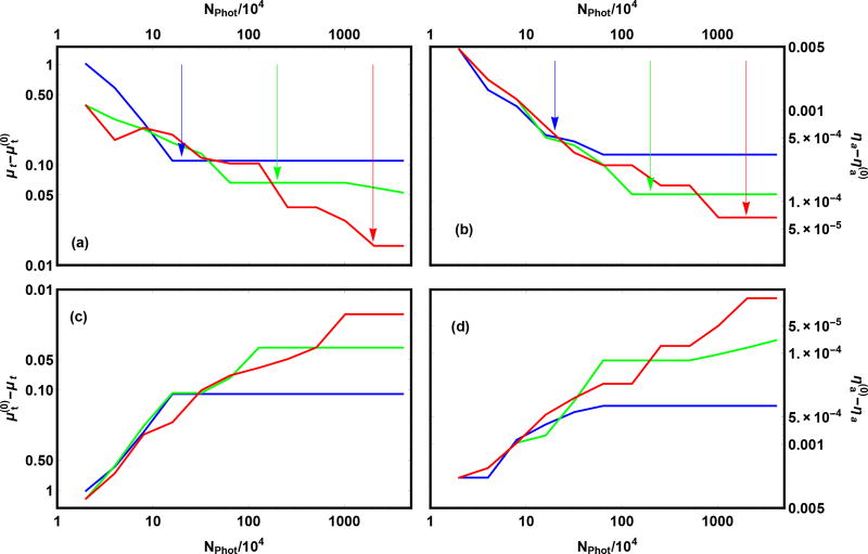
The profile log likelihood method takes into account both Monte Carlo uncertainty and experimental uncertainty. For this test, we use the forward model to generate simulated experimental data. For the results shown in Fig. 2, the forward model exactly matches the inverse model so the “experimental” uncertainty is entirely due to the finite number of Monte Carlo samples in preparing the “experimental” data. When the number of Monte Carlo trials used to determine the best fit parameters increases from a small number to a large number we expect the bounding box will shrink at first; subsequently, when the number of Monte Carlo trials in the inverse increases past the number used to simulate the experimental data, then the size of the bounding box will asymptote to some value determined by the noise in the experiment. Additionally, we expect that the bounding boxes for less noisy “experimental” data will be smaller than those for more noisy data. All of these features are seen in Fig. 2, and the cross-over occurs when the number of photons used for the inverse problem equals the number used in simulating the data.

Fig. 2.

Search boxes for three trials with simulated data. The bounds of the search box relative to the exact answer are shown: (a) upper bound for μ_t, (b) upper bound for η_a, (c) lower bound for μ_t, and (d) lower bound for η_a. The blue, green, and red curves correspond to simulated data created with 2 · 10⁵, 2 · 10⁶, and 2 · 10⁷, photons respectively, as indicated by the vertical arrows. The value N_phot corresponds to the number of photons used in each of 12 iterations, starting from 2 · 10⁴ and doubling 11 times to 4.096 · 10⁷. The simulation used the parameters ${\mu }_s^{(0)}=3{\text{ mm}}^{-1}$ and ${\mu }_a^{(0)}=0.01{\text{ mm}}^{-1}$ corresponding to ${\mu }_t^{(0)}=3.01{\text{ mm}}^{-1}$ and ${\eta }_a^{(0)}=0.003322{\text{ mm}}^{-1}$, thickness t = 4.76 mm, index of refraction n = 1.487, and asymmetry parameter g = 0.621.

3.3.3. Profile Log Likelihood Optimization

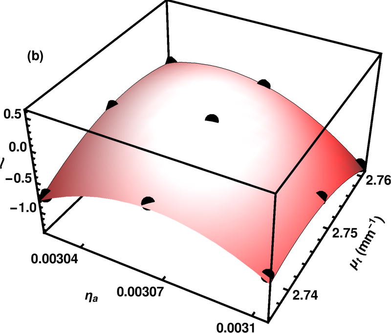
We illustrate the log likelihood surfaces for the inverse problem with the experimental data of λ = 805 nm and t = 10.12 mm. At the final iteration, we find the maximum log likelihood value among those calculated on the grid and fit points in a 3×3 neighborhood centered on that point to a quadratic. The fit is seen to be excellent, as illustrated in Fig. 3.

Fig. 3.

The quadratic approximation to the likelihood surface is obtained from a fit to the importance sampling results on a 3×3 grid including the maximum likelihood point found on the grid.

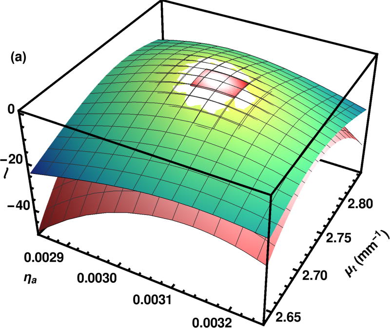
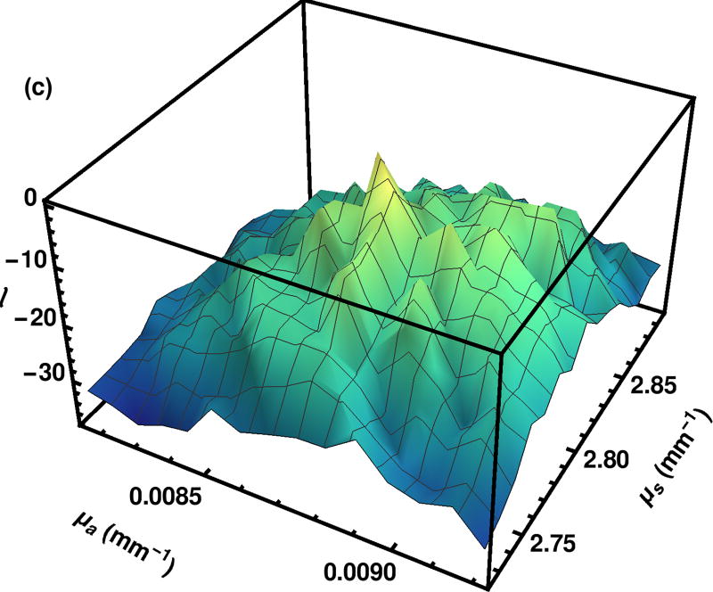
The set of points for the quadratic fit are in the center of the likelihood surfaces, shown in Fig. 4. Although the quadratic fit is good near the top, over the full region, the quadratic surface falls off more quickly than the actual likelihood calculated with importance sampling.

Fig. 4.

The log likelihood surface ℓ as calculated by the importance sampling method is shown in green tones. The quadratic approximation to the same surface is shown in peach tones. The small patch at the top of the graph is the context for the whole surface shown in Fig. 3.

The smoothness of the surface generated by importance sampling eases the process of finding a quadratic fit to the maximum. For comparison, a log likelihood surface formed using our algorithm with the exception that the log likelihood is evaluated independently at each grid point rather than using importance sampling, as shown in Fig. 5.

Fig. 5.

Log likelihood surface as calculated by the explicit grid method. The region shown was calculated with 2.56 · 10⁶ photons per grid point with the region selected on the eighth iteration building up from 2 · 10⁴ photons per grid point over a much larger region.

3.4. Comparison Algorithm: Particle Swarm Optimization

The PSO update equations are

$$V_{i+i}=w_i{V}_i+c_1{ℛ}_1(X_{\text{cl}}^{(\text{opt})}-X_i)+c_2{ℛ}_2(X_{\text{gl}}^{(\text{opt})}-X_i)$$ (11)

$$X_{i+i}=X_i+V_{i+1}$$ (12)

where i is the 0-based iteration number, X_i is the position of a particle at iteration i (the particle index is suppressed), V_i is the “velocity” (or step size) of the particle, $X_{\text{cl}}^{(\text{opt})}$ is the best position achieved up to and including iteration i for any particle in the cluster of a particle, $X_{\text{gl}}^{(\text{opt})}$ is the best position achieved up to and including iteration i for any particle in any cluster, ℛ₁ and ℛ₂ are two uniform random deviates on [0, 1), and c₁ = 0.2 and c₂ = 0.8 are constants, following Ref. [30]. We also follow the reference in varying the weight w_i linearly from 0.9 at iteration 0 to 0.5 at iteration 10 with the value remaining constant thereafter. We operate in the space of the logarithm of μ_a and μ_s. The 27 points are initially spread out in 9 clusters populating a grid from 0.001 mm⁻¹ ≤ μ_a ≤ 0.007 mm⁻¹ and 1 mm⁻¹ ≤ μ_s ≤ 4 mm⁻¹. Within each cluster, the search space is temporarily scaled to the unit square, then the points are arranged on a circle with 120° spaces and a radius of 0.05. The particles are not required to remain in the original bounding box. Part of the motivation for working in the space of the logarithm is to ensure μ_a > 0 and μ_s > 0 throughout the process.

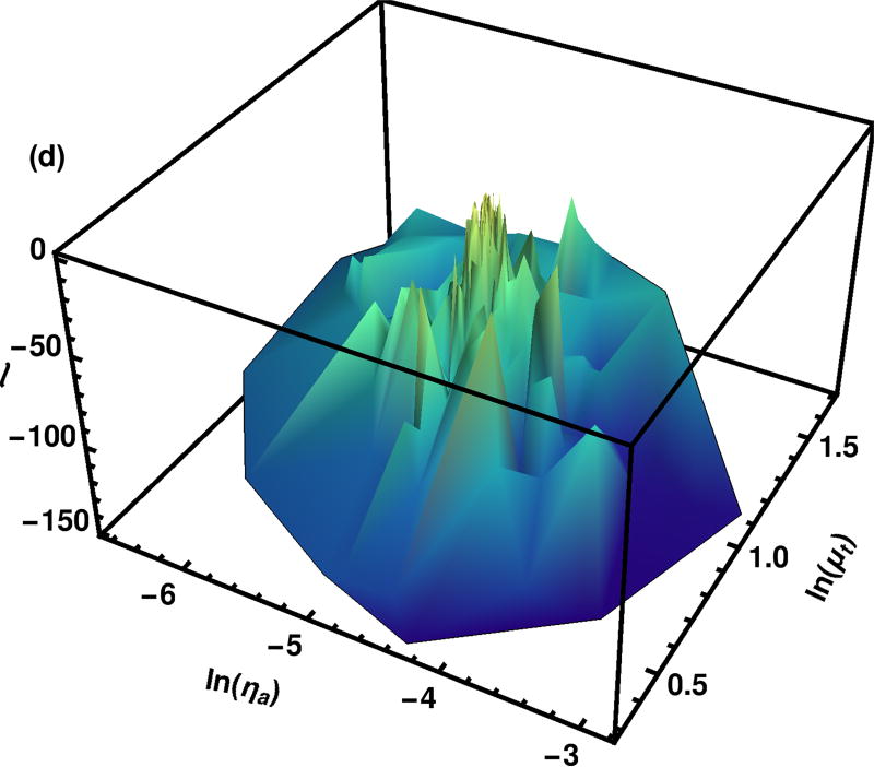
The log likelihood surface found during Particle Swarm Optimization is shown in Fig. 6. Although there is a clear maximal region shown in the graph, there is a large amount of variation in the log likelihood calculated by the various points. The region shown in Fig. 6 is many, many times the size of that shown in Fig. 5.

Fig. 6.

Log likelihood surface as calculated by the Particle Swarm Optimization. Each point was calculated with 1.28 · 10⁶ photons. All of the points evaluated at any iteration are shown. A constant number of photons is used at every iteration.

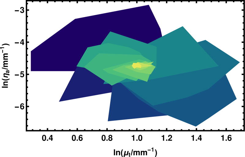
To illustrate how the swarm of particles converges, in Fig. 7 we plot the convex hull of the points at each iteration, starting from the iteration 1 (which is not the initial position, iteration 0), through iteration 17 at which point the size of the swarm has substantially stabilized. The shrinking of the regions is evident, as is the “swarm” nature of many points testing one side of the ultimate optimum or another as they home in on the best value.

Fig. 7.

The convergence of the Particle Swarm Optimization algorithm is illustrated in this figure. Each region in the convex hull of the points in the swarm at a given iteration. The first iteration is purple and is placed at the bottom of the stack. Higher iterations are places upon it with the color tending toward yellow. Iterations fifteen and higher are represented in the same color yellow. The variables are plotted in the natural logarithm because the PSO operates in this space.

4. Comparison to Experiment

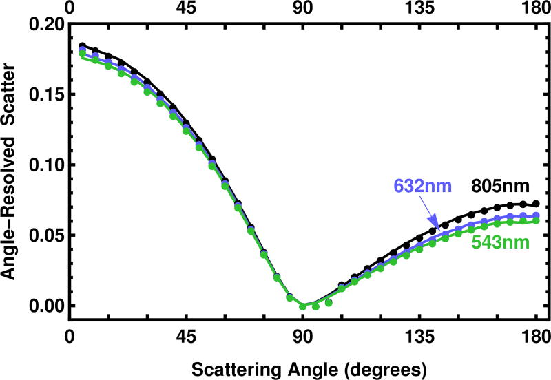
Going forward, all results refer to our importance sampling algorithm unless stated. The angle-resolved scatter is show in Fig. 8. Although the pattern of the angle-resolved scatter for the three wavelengths shown is quite similar, it is clear that the predictions are sufficiently different to clearly distinguish them.

Fig. 8.

Angle-resolved scatter is given for three wavelengths, 543 nm (green), 632 nm (orange), and 805 nm (black) for the sample with a thickness t = 6.10 mm. The values of μ_a and μ_s are shown in Fig. 9. Experimental points are given as dots. For convenience, the value of 0 was assigned to the measurement at 90°. The solid line is the prediction at the best fit found by the profile log likelihood importance sampling algorithm.

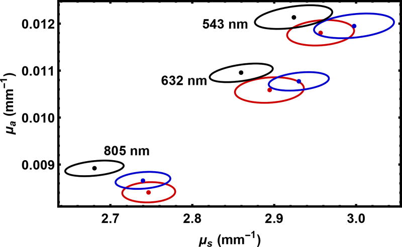
This point is illustrated more formally in Fig. 9 where we present our point estimates and confidence regions for the 9 samples. In principle, we expect the values of the scattering parameters to be the same as the thickness is varied. This is not quite true, suggesting an unresolved material preparation or other experimental issue at the level of about 3%. In this paper, we treat the experimental results as given, hence the discussion is restricted to the statistical precision which the algorithm can achieve with real data. It is notable that the full set of results in Fig. 9 was generated with about 10 minutes of computer time on a modest 4 processor desktop.

Fig. 9.

Point estimates and 95% confidence regions for 9 measured samples. The wavelengths are indicated, and the sample thickness is 6.10 mm (red), 8.10 mm (blue), and 10.12 mm (black).

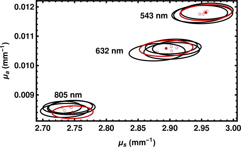
The effect of varying the random seed is shown in Fig. 10. The variation in the choice of the seed is smaller than the effect of varying the wavelength experimentally. Moreover, each of the five solutions for each of three experimental conditions lies in the 95% confidence intervals of each of the other solutions.

Fig. 10.

Effect of the choice of the random seed is shown. The point estimates and 95% confidence regions shown with solid red circles and solid red lines are replotted from Fig. 9 for the sample thickness 6.10 mm. The hollow red circles and black lines represent other solutions which differ only in the seed of the random number generator.

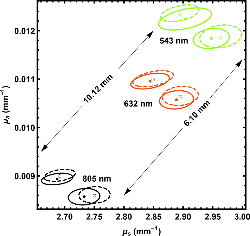
As noted above when presenting Eq. (3) and Eq. (4), we keep track of the finite radius of the source to the detector. As shown in Fig. 11, this proves to be about a 1% effect. This effect is small enough to be neglected in most cases, but large enough to be included in standards work.

Fig. 11.

The effect of the finite detector radius is shown. Pairs of results are generated with the same seed for for λ = 543 nm, 632 nm, and 805 nm with the detector at a finite radius (solid circles and 95% confidence contours) and at an effectively infinite radius (hollow circles and dashed contours). The results are given for samples of two thicknesses, 6.10 mm and 10.12 mm as marked in the figure.

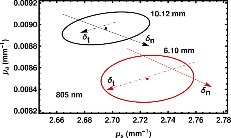
Although we do not formally include the thickness t or the index of refraction n in our log likelihood, nevertheless we may see their effects through a sensitivity analysis, shown in Fig. 12. The effects of the uncertainty in the thickness and index of refraction are comparable to other measurement uncertainties in the problem.

Fig. 12.

The effect of changing the thickness and the index of refraction is given for a wavelength of 805 nm. The red and black symbols refer to the sample with a thicknesses of 6.10 mm and 10.12 mm, respectively. The solid dots and ellipses are carried over from Fig. 11. The solid and dashed arrows describe calculations with the the index of refraction and the sample thickness respectively changed at the k = 2 level as quoted in the text. The tails of the arrows represent lowering the central value at the k = 2 level and the heads of the arrows represent raising the central value at the k = 2 level. The shaft of the arrow is a guide to the eye.

The uncertainty in thickness cannot resolve the discrepancy between the samples with nominal thicknesses of 6 mm and 10 mm because it does not bring the uncertainty regions closer together. The uncertainty in the index of refraction could resolve the discrepancy, although it is at least as likely that there is a small difference in properties between the samples or other factors are in play.

5. Computational Issues

5.1. Range of Validity

As mentioned in the introduction, the experimental program has been centered on obtaining medical phantoms with scattering properties comparable to that of human skin. One question is whether the method proposed here is particularly specialized to that range of parameters, and, in particular, whether it can be extended into the single-scatter regime.

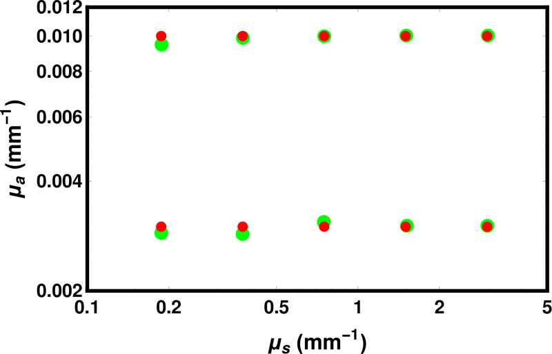
In Fig. 13, we show the effect of varying μ_s from 0.1875 mm⁻¹ to 3 mm⁻¹ in steps of a factor of 2. as well as taking μ_a to be 0.003 mm⁻¹ and 0.010 mm⁻¹. The results show that the program is capable of tracking the ground truth over this range. The probability of passing directly through the detector is 0.32 for the longest scattering length considered, which approaches the single-scatter regime. As a large number of photons accumulate in the unscattered bin, the assumption of equal noise for each bin becomes increasingly doubtful, suggesting our likelihood model would need to be refined.

Fig. 13.

Comparison of maximum likelihood estimates (large green circles) with ground truth (small red circles) for several values of μ_a and μ_s with fixed parameters g = 0.621, t = 6.10 mm, and n = 1.5. The ground truth was created with the forward program using 2¹² · 10⁴ = 40 960 000 photons, vs. 2⁷ · 10⁴ = 1 280 000 photons in the final round for the inverse problem.

5.2. Timing

Because this paper is principally about algorithms, we close with the timing comparison of our method to some alternatives given in Table 3. First, considering the forward model, our implementation is comparable in speed to the benchmark MCML code. Our lower reported number does not necessarily reflect any improvement because of small differences in implementations. For example, MCML uses particle splitting during the Fresnel reflection/transmission event whereas we simply pick one alternative. By implementing OpenMP (OMP) for our algorithm, allowing the use of parallel random number generation, we gain a factor of 2.5 with 4 processors. Finally, we are able to predict the results on a 15 × 17 grid in η_a, μ_t at a cost of a factor of 3.0 compared to predicting on a single point.

Table 3.

The run time is given for N_phot = 1.28 · 10⁶ Monte Carlo trials, which is our principal operating point in the paper. for the sample with t=6.10 mm and λ = 805 nm. The number of processors used is N_proc. The notation “Fwd” means that only the forward problem is solved (i.e., the ARS is found for one set of parameters) “Inv” refers to the inverse problem (i.e., solving for a set of parameters). The number of iterations is quoted as the number necessary to reach convergence. The number of times the 1.28 · 10⁶ Monte Carlo trials were performed in the final iteration is reported as N_eval. In the case of PSO, this number of evaluations is performed at every iteration. In the present methods, the number of Monte Carlo trials increases from 2 · 10⁴ to the final value by doubling at each iteration. The times refer to runs on a Dell Optiplex 9010 AIO computer with an Intel i5-3570S quad-core processor running at 3.10 GHz. The present explicit grid method is estimated because it was implemented in a scripting language on a different computer.

		Nproc		Niter	Neval	time (s)
MCML [40]	C	1	Fwd	1	1	47
Present single point estimate	C++	1	Fwd	1	1	33
Present single point estimate	C++/OMP	4	Fwd	1	1	13
Present importance sampling	C++/OMP	4	Fwd	1	1	39
Particle Swarm Optimization	C++/OMP	4	Inv	17	27	4748
Present explicit grid	Est.	4	Inv	7	255	5300
Present importance sampling	C++/OMP	4	Inv	7	1	75

Turning to the inverse problem, our solution takes 1.9 times as long as the forward problem, in line with our estimate given earlier that the total time-to-solution comparing the full problem to the evaluation on the last grid. Although we have 7 iterations, the number of photons used in the earlier iterations doubles, so half the time is spent on the final iteration. Operations other than Monte Carlo sampling take a negligible amount of time. Because the time-to-solution is dominated by the Monte Carlo sampling, the explicit grid method for the inverse problem is also estimated to take about 70 times longer than the importance sampling method.

Particle Swarm Optimization requires about the same number of Monte Carlo samples evaluations as the explicit grid method, and hence the time is comparable. the importance sampling method is 64 times faster than Particle Swarm Optimization which is a key result of this manuscript.

6. Conclusions

On the experimental side, we demonstrate that the STARR is capable of delivering measurements which contribute about 2% to the uncertainty of measurement of the optical scattering parameters μ_a and μ_s. Such precision may be compared, to uncertainties of 0.5% for μ_a and 1.5% for ${\mu }_s^{\prime }$ were reported using a time-dependent method, [7] about 2% using a CW method with several optical fibers receiving scattered photons, [10] and 3% using a combination of broad-band and steady-state reflectance methods. [8] Uncertainties associated with the Inverse Adding Doubling method [15] have been reported recently to be 10% or more for human tissue phantoms. [17, 18]

Although STARR integrates over a much smaller solid angle than an integrating sphere measurement would, it provides a more detailed view of the angular distribution. The low-noise results allow a reasonably fine discrimination between values of (μ_a, μ_s) even though the detector subtends a modest solid angle. We emphasize that the 2% uncertainty represents only part of the uncertainty budget, and factors such as surface roughness, form errors, polarization, uncertainty in parameters such as t, g, and n are not included in the analysis of this paper, except to the extent that the effect of uncertainty in n and t was addressed by a sensitivity analysis. We demonstrated that the effect of sample thickness and finite detector radius is at the level of 1% or less.

Algorithmically, we combine several ideas into a rapid computer program. First, we take the log likelihood to be our object function. We use this two ways: (a) as a guide for shrinking the search region, providing a principled method for discarding ranges of parameters, and (b) to produce not only maximum likelihood estimates but confidence regions as well. Second, we increase the number of Monte Carlo samples by factors of two as the search region shrinks. Thus we take advantage of the fact that some parameters in a large search region are bad enough to be ruled out with relatively few Monte Carlo trials. By doubling the number of Monte Carlo samples at each iteration, fully half of the trials occur on the final iteration where we make our likelihood predictions. Third, we take advantage of the cylindrical symmetry of the problem so that every photon which leaves the sample is scored in the detector. Fourth, we use a parallel random number generator to permit parallel processing. Fifth, we use importance sampling to make predictions not only at a single point, but over a whole grid of values. In a related point, we work with variables which are related by independent probability distributions, so the computational cost at each interaction is linear in the number of possibilities in 1D although score each photon on a 2D grid. The principle would hold with a multi-layer structure or if other parameters such as g and n were varied.

Using all of these techniques, we can create a 15×17 grid with 255 evaluated points at a computational cost of 3 standard Monte Carlo evaluations and we can solve an inverse problem at 6 times the cost of evaluating the forward problem at a single point. Through this combination of ideas, we are able to implement a program to solve the inverse problem of optical parameter estimation in single layers in 75 seconds on a desktop computer—fast enough to create real-time solutions in experimental laboratories.