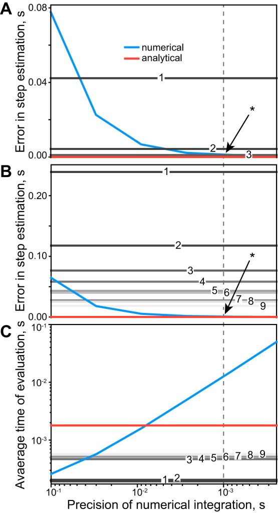
Fig. 3.

The comparison of analytical and numerical solutions. The measures of numerical (blue), analytical (red), and analytical approximations of different orders (shades of gray with order numbers) are plotted as functions of numerical precision, where the dashed line indicates the most relevant for real-time simulation precision of 1 ms. A: full cycle error in the estimation of phase transition times using the 1% neighborhood of the optimal solution. Because the higher orders of approximations provide the same high precision as the cubic approximations, powers τ4–τ9 are not displayed. B: similar to A; the errors are shown for the random distribution of parameters. C: average central processing unit time needed to calculate a full step period of 1.25 s (average from Halbertsma’s equations) in Python/NumPy implementation. The data presented in all subplots were averaged over 105 trials.
