
Figure 1. Stimulus generation and modulation power spectrum.
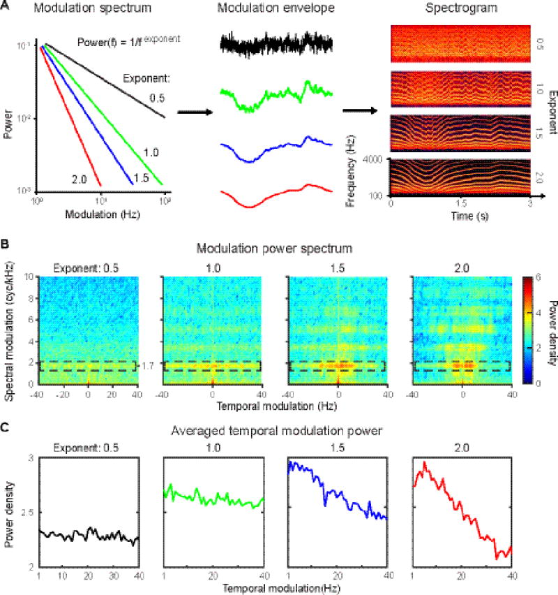
A, Schematic plot of stimulus generation. Left panel: schematic plot of modulation spectra used to generate modulation envelopes. The color code represents the spectra of different exponents. Black: 0.5; green: 1.0; blue: 1.5; red 2.0. Middle panel: modulation envelopes generated using the four different exponents. (Color code as in the modulation spectra.) Right panel: spectrograms of the four ‘frozen’ stimuli (see Methods) used in the experiment. Sound files of the stimuli can be accessed here: http://edmond.mpdl.mpg.de/imeji/collection/kZalRMtxa19mlRyG. B, Modulation power spectra of the four frozen stimuli. The dashed boxes show increased power density at a spectral modulation of around 1.7 cycles per 1000 Hz in the stimuli. C, The averaged temporal modulation spectrum. The averaged temporal modulation was computed by averaging along the spectral modulation dimension of the modulation power spectrum (in B). From left to right, the averaged temporal modulation spectrum of each stimulus becomes steeper as the exponent increases. Note that there are no prominent peaks in the averaged temporal modulation spectra that indicate regular modulations centered at a narrow frequency band.