Figure 2:

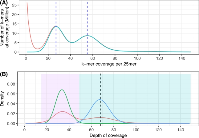
Depth of coverage analysis. (A) Histograms of k-mer frequencies in the filtered read data for k = 25 (red) and GenomeScope modeling equation on H. impetiginosus (blue). The x-axis shows the number of times a k-mer occurred (coverage). The vertical dashed dark blue lines correspond to the mean coverage values for unique heterozygous k-mers (left peak) and unique homozygous k-mers (right peak). (B) Density plot of read depth based on mapping all short fragment reads back to the assembled scaffolds (red). Left peak (at depth = ×34) corresponds to regions where the assembler created 2 distinct scaffolds from divergent putative haplotypes. The right peak (at depth = ×67) contains scaffolds from regions where the genome is less variable, allowing the assembler to construct a single contig combining homologue sequences. Histograms of Poisson modeling for read depth in the assembly (green, lambda = 34; blue, lambda = 67) are shown.