Quantifying within-plant spatial heterogeneity in carbohydrate availability in cotton using a local-pool model

Abstract

Background and Aims

Within-plant spatial heterogeneity in the production of and demand for assimilates may have major implications for the formation of fruits. Spatial heterogeneity is related to organ age, but also to position on the plant. This study quantifies the variation in local carbohydrate availability for the phytomers in the same cohort using a cotton growth model that captures carbohydrate production in phytomers and carbohydrate movement between phytomers.

Methods

Based on field observations, we developed a functional–structural plant model of cotton that simulates production and storage of carbohydrates in individual phytomers and transport of surplus to other phytomers. Simulated total leaf area, total above-ground dry mass, dry mass distribution along the stem, and dry mass allocation fractions to each organ at the plant level were compared with field observations for plants grown at different densities. The distribution of local carbohydrate availability throughout the plant was characterized and a sensitivity analysis was conducted regarding the value of the carbohydrate transport coefficient.

Key Results

The model reproduced cotton leaf expansion and dry mass allocation across plant densities adequately. Individual leaf area was underestimated at very high plant densities. Best correspondence with measured plant traits was obtained for a value of the transport coefficient of 0.1 d⁻¹. The simulated translocation of carbohydrates agreed well with results from C-labelling studies. Moreover, simulation results revealed the heterogeneous pattern of local carbohydrate availability over the plant as an emergent model property.

Conclusions

This modelling study shows how heterogeneity in local carbohydrate production within the plant structure in combination with limitations in transport result in heterogeneous satisfaction of demand over the plant. This model provides a tool to explore phenomena in cotton that are thought to be determined by local carbohydrate availability, such as branching pattern and fruit abortion in relation to climate and crop management.

INTRODUCTION

Woody plants need to cope with a wide range of stresses and disturbances through adjustment of their strategies for carbon utilization and allocation (Dietze et al., 2014). Growth and reproduction represent competing demands for a finite supply of carbohydrates. Within a plant, organs compete for carbohydrates for their growth. The majority of carbohydrate used by vascular plants is not used at the site of assimilation (source) but is transported to areas of active growth (sinks) (Savage et al., 2016). Upper leaves send assimilates to the developing shoot apex, lower leaves transport assimilates to the roots, and middle leaves transport assimilates bidirectionally (Watson and Casper, 1984). In a wide range of species, fruits have been shown to receive carbon primarily from nearby leaves (Wardlaw, 1990). The pattern of assimilate movement in the plant is a crucial determinant of its growth and performance, and is therefore of interest in the analysis and improvement of crop performance.

Cotton is a perennial species, but it is widely grown as an annual in agriculture. The allocation of carbohydrates is a major factor determining yield formation. To maximize cotton yield, farmers adopt a package of agronomic practices (e.g. high plant density, chemical growth regulators and pruning of vegetative branches) that suppress vegetative growth and promote carbohydrate allocation to fruits. Fruit abortion in cotton, which can be as high as 70 %, depends on carbon availability, not only as an energy source for growth but also as a signal of plant resource status (Guinn, 1982; McDowell et al., 2011). While many consequences of biomass allocation in cotton have been reported (Sadras et al., 1997), transport rate and partitioning of sugars can only be measured with labelled C (Minchin and Thorpe, 2003). Limited possibilities exist to quantify the local status of carbohydrates at organ level over the plant structure, and this hampers our understanding of how cotton plants allocate the available carbohydrate, and thus how cotton growth and yield are determined. This is where plant modelling can play a role.

Numerous simulation models have been developed to better understand cotton responses to crop management (Baker et al., 1983; Hearn, 1994; Zhang et al., 2008). These models simulate development, photosynthesis, dry mass allocation and yield formation in relation to cultivar (Reddy and Baker, 1988), environment (Reddy and Baker, 1990) and management (Yang et al., 2008). They operate at the level of the crop canopy, in contrast to functional–structural plant (FSP) models, which simulate ‘the development over time of the 3D architecture or structure of plants as governed by physiological processes which, in turn, depend on environmental factors’ (Vos et al., 2010; Evers, 2016). Functional–structural plant modelling is a suitable tool for simulating how temporal and spatial heterogeneity in light interception and assimilate production affect yield formation. Functional–structural plant models of cotton have been developed to investigate how the fruit distribution in the canopy is affected by water, N and C stress (Hanan and Hearn, 2003). These models have also been used to examine plant plasticity in response to plant density and plant configuration (Dauzat et al., 2008; Mao et al., 2016) and to explore the structural responses of cotton plants to plant density and growth regulators (Gu et al., 2014). A number of these models simulate carbohydrate production and allocation (Baker et al., 1983; Hearn, 1994; Zhang et al., 2008). They all assume a plant-wide (common or global) pool of assimilates and determine the amounts allocated to different organs using empirical allocation models (Goudriaan and Van Laar, 1994) or a relative sink-strength approach (Heuvelink, 1996). Such an approach is, however, at odds with known patterns of assimilate production in the plant, and the likely constraints on long-distance transport of carbohydrate within the plant structure. Functional–structural plant modelling can take into account the within-plant spatial heterogeneity in assimilate production and the consequences of this heterogeneity for meeting the demand of organs. Such modelling has been employed to simulate the variability of fruit growth in peach (Allen et al., 2005), kiwi fruit (Cieslak et al., 2011) and apple (Pallas et al., 2016). but it has not been considered for cotton.

There is a large heterogeneity in weight and quality of cotton bolls at different positions within the plant. Seventy to ninety percent of total harvestable bolls come from the inner canopy, defined as the first and second sites on every fruiting branch (Wang et al., 2016). Cohorts contain organs of nearly the same age (Stewart and Sterling, 1988). As the global-pool model determines carbohydrate allocation using sink strength, which is solely dependent on organ age, a global-pool simulation would map a homogeneous distribution of local carbohydrate availability for the fruits in the same cohort and thus the same probability of fruit abortion. However, such a pattern is not supported by empirical data on boll growth (Wang et al., 2016). Fruit growth and quality have been demonstrated to be related to local carbon availability (Berüter and Droz, 1991; Gómez-Cadenas et al., 2000; McFadyen et al., 2011). This variability has been reported not only in fruit trees such as peach (Génard, 1992), kiwi fruit (Piller et al., 1998) and grapevine (Pallas et al., 2010) but also in annual crops such as soybean (Stephenson and Wilson, 1977) and tomato (Hocking and Steer, 1994). The leaf subtending a cotton fruit is the major source of carbohydrate, supplying 60–87 % of the carbohydrate requirement of the fruit, while the remainder is supplied by other phytomers (Constable and Rawson, 1980a). The localization of supply and demand needs to be accounted for when investigating the dynamics of the distribution of carbohydrate within the developing cotton plant using a modelling approach (Lacointe, 2000; Mathieu et al., 2009).

Here we present a cotton model that integrates carbon assimilation, transport and accumulation at the level of individual phytomers. The purpose of this study is to provide an approach for quantifying and explaining the heterogeneity of local carbohydrate availability for phytomers that belong to the same cohort but appear at different positions on the plant. For this purpose, we performed the following analyses: (1) we characterized the fruiting pattern of cotton experimentally, to show that a global-pool view that would result in similar allocation across organs of the same age (and demand) is not appropriate for cotton; (2) we tested the model predictions of cotton growth by comparison with experimentally observed total leaf area, total above-ground dry mass, dry mass distribution along the main stem and allocation fractions to each type of organ at the plant level at a range of plant densities; (3) we compared predicted and observed carbohydrate transport to calibrate the carbohydrate transport coefficient; and (4) we provide model support for the experimentally observed heterogeneity of carbohydrate supply for phytomers in the same cohort using the local-pool model.

MATERIALS AND METHODS

Experiments

Field experiments were carried out in 2014 and 2015 at the Cotton Research Institute of the Chinese Academy of Agricultural Sciences, Anyang, Henan, China (36′07″ N, 116′22″ E). The soil properties of the experimental field have been described in Gu et al. (2014). Cotton (Gossypium hirsutum ‘Lumian 28’) plants were grown at three plant population densities: 1.5, 7.5 and 13.5 plants m⁻². The experiments were laid out as a randomized complete block design with four replicates. Cotton plants were sown on 1 May 2014 and 18 April 2015, and were harvested on 4 October 2014 and 1 October 2015. Mature bolls were picked at the beginning, middle and end of October. Destructive measurements were made on three plants that were randomly sampled in each plot every 2 weeks from seedling until harvest to measure organ dry weight. We divided a cotton plant according to the main stem rank first and separated leaves, stems and fruits. Size of organs was measured and organs were dried to constant weight at 75 °C for 48 h (Gu et al., 2014). The duration of growth of an organ was calculated as the period from its initiation to the maximum size. The mass of organs was measured to parameterize the sink-strength functions (see the Light absorption, photosynthesis and respiration section, below). In 2015, growth duration, final dry mass and phytomer rank on the main stem and the fruiting branch were measured for each boll on 20 plants per plot. Data from 2015 were used for parameterizing the model while data for 2014 were used for testing the model. Temperature data were obtained from the National Meteorological Information Center of the China Meteorological Administration (data.cma.cn).

Characterizing fruiting pattern

The fruiting pattern was described by calculating the probability of a harvestable boll for each phytomer. This probability was calculated as the ratio of the total number of harvestable bolls observed on that phytomer to the total number of measured plants (80), i.e. assuming that the phytomer was (potentially) present on each of the 80 plants. For visualization we focused on the primary fruit branches and ignored fruits on secondary or higher-order fruiting branches. The distribution of harvestable bolls was visualized using the ggplot2 package of the R programming language (Wickham, 2009). Our analysis focused on answering the question whether phytomers that had been initiated at the same time, and were therefore in the same age cohort, had the same or a different probability of having a harvestable boll, and whether this probability was linked to local carbohydrate supply. The first cohort contained the oldest fruits, which were located near the base and centre of the main stem, whereas the last cohort consisted of the latest fruits, which were initiated at the top and periphery of the main stem (Stewart and Sterling, 1988).

General features of CottonXL

The developed model was based on CottonXL, an existing cotton model, which describes the architectural development of cotton plants in relation to plant densities and effects of a growth regulator but lacks eco-physiological processes (Gu et al., 2014). In the current study, the model was extended with modules for carbohydrate production, transport and consumption as well as organ biomass growth. The cotton plant was simulated as a network of phytomers, in which a vegetative phytomer consists of an internode and a leaf while a fruiting phytomer also includes a fruit. The rate of production of new phytomers was determined by the phyllochron (thermal time between appearances of successive leaf blades). The internode, leaf and fruit of one phytomer were initiated simultaneously. Cotton plants produce vegetative branches at main stem phytomers 4–7 and fruiting branches at main stem phytomers 8 and upwards, as well as on the vegetative branches (secondary fruiting branches) (Supplementary Data Fig. S1). The appearance and architecture of organs were simulated descriptively based on experimental data. Organ biomass growth was simulated mechanistically based on light capture and the production and distribution of carbohydrates.

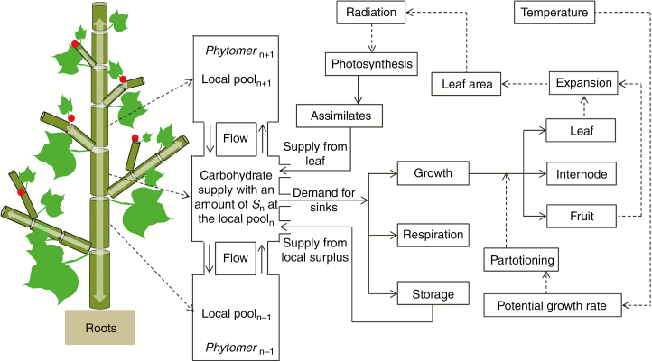
Internodes functioned solely as sinks for carbohydrates, whereas leaves and fruits functioned as sinks for the duration of their growth but as sources of assimilates during their entire lifespan, due to their large photosynthesizing bracts. Initial growth of the plant was supported by the seed endosperm mass. Instead of calibrating the seed mass to provide ample resources to establish the seedling, we used a measured value of seed mass. At each time step and for each phytomer, the carbohydrates provided by the leaf, fruit and local assimilate pool were transported between connected phytomers depending on the difference in carbohydrate level and the transport coefficient (Fig. 1 and the Transport between connected phytomers section, below). The root system was modelled as a single sink compartment and was not represented architecturally. It received carbohydrates from upper neighbouring phytomers for maintenance and growth.

Fig. 1.

Schematic representation of a cotton plant as implemented in the FSP model. Full-line arrows are material flows and dashed-line arrows are information flows. Cotton is modelled as a set of phytomers. Each phytomer is composed of a leaf (green lamina), an internode (dark green cylinder) and a fruit (red point). Fluxes of carbohydrate are represented by white arrows in the internode and are governed by the difference in supply between neighbouring internodes and the transport coefficient. The photosynthetic organs are leaves and bracts of fruits in the model.

The model was implemented using the GroIMP platform (Hemmerling et al., 2008; Kniemeyer, 2008). The detailed functionality of the model is outlined in the following sections. Light capture, photosynthesis, respiration, allocation and architectural development were computed at a daily time step, whereas carbon transport was solved with an adaptive step size (see Transport between connected phytomers section, below). All processes at different times were combined to form a hybrid model in which the amount of carbohydrates produced via photosynthesis was calculated once per day, and then the amount available from this daily photosynthesis and storage was transported over the plant using an adaptive step size over a daily time period to calculate the distribution of assimilates over all the phytomers in the plant. The carbohydrates allocated to each phytomer were distributed over organs within the phytomer according to distribution ratios. The updated organ sizes then determined light interception in the next time step, continuing until the end of the simulation.

Light absorption, photosynthesis and respiration

The simulated scene in the radiation model of GroIMP was built with a combination of an arc of light sources representing the course of direct light during a day and a dome of light sources representing diffuse light (Evers et al., 2010; Evers, 2016). The direct light intensity of each source point was calculated using mathematical formulae (Spitters et al., 1986; Goudriaan and Van Laar, 1994). This improved the accuracy of incoming radiation over the growing season as compared with the radiation model in the previous version of CottonXL, in which we used a single light source for direct radiation with a fixed total incoming radiation of 25 MJ m⁻² d⁻¹ (Gu et al., 2014; Mao et al., 2016). The diffuse light power was simulated by using a fixed function of elevation angle (Evers et al., 2007). Daylength, azimuth and solar elevation angle were used to determine the position of each direct light source, and were calculated based on latitude and day of the year. Photosynthetically active radiation (PAR) at the top of the canopy was expressed as photosynthetic photon flux density (μmol photons m⁻² s⁻¹). Stochastic path tracer principles were used to determine the absorption, reflection and transmission of PAR for a plant organ, resulting in an organ-level calculation of the distribution of PAR. Leaf reflectance and transmittance of cotton were set to 0.11 and 0.076, respectively (more details are given in Mao et al., 2016).

Photosynthetically active radiation absorbed by a photosynthetic organ was used to calculate the photosynthesis rate using the negative exponential photosynthesis–light response curve (Goudriaan and Van Laar, 1994):

$$A= A_{max}(1-e^{-\epsilon I/A_{max}})$$ (1)

where A (μmol CO₂ m⁻² s⁻¹) is the photosynthesis rate, A_max (μmol CO₂ m^−m s^−s) is the maximum photosynthesis rate in saturating light, I (μmol photons m^−h s^−s) is the PAR intercepted by the organ and ε (μmol CO₂ μmol⁻¹ photons) is the initial light use efficiency.

In a canopy, A_max typically follows the nitrogen gradient. Since nitrogen economy is not part of this model, we adopted an empirical relationship between A_max and the gradient of the fraction of PAR intercepted (I), using a power law (Niinemets and Anten, 2009):

$$A_{max}=A_{max0}{\left(\frac{I}{I_0}\right)}^{0.4}$$ (2)

where I₀ (μmol photons m^−m s^−s) is the PAR at the top of the canopy, A_max0 (μmol CO₂ m^−m s^−s) is the maximum photosynthesis rate at the top of the canopy, where I/I₀ equals 1. The photosynthesis rate (A) was converted to daily assimilate production (S_d, mg CH₂O d⁻¹) using the following conversion formula without taking the daily path of the sun into consideration:

$$S_d=A \times a_l \times d \times 3600 \times 30 \times {10}^{-0}$$ (3)

where a_l (m²) is the area of a photosynthetic organ and d is the day length (h). Maintenance respiration rate (mg CH₂O d⁻¹) was calculated as a fraction (r_organ) of the organ biomass (M_organ, mg) without taking an effect of temperature into consideration.

The potential growth rate determines the sink strength of each organ. The potential growth rate D (mg CH₂O mg organ⁻¹ (°C d)⁻¹) at age t (°C d) of a growing organ was calculated using the β growth function (Yin et al., 2003):

$$D= \frac{t_e-t}{t_e-t_m}{\left(\frac{t}{t_m}\right)}^{\frac{t_m}{t_e-t_m}}{c}_m$$ (4)

where c_m (mg (°C d)⁻¹) is the maximum growth rate, which is achieved at age t_m, and t_e is the end time of the growth period. We calculated c_m as:

$$c_m=\frac{2t_e-t_m}{t_e\left(t_e-t_m\right)}{\left(\frac{t_m}{t_e}\right)}^{\frac{t_m}{t_e-t_m}}{W}_{max}$$ (5)

where W_max (mg) is the potential maximum dry mass of an organ. The potential maximum organ mass was estimated using measurements at the lowest plant density of 1.5 plants m⁻², at which plant–plant competition was minimal. The growth duration (t_e) of individual internodes and leaves was determined by measuring the duration of organ mass increase. The growth durations of the root system and fruits were taken from the literature (Table 1). The age at which maximum growth rate was reached (t_m) was assumed to be half of the growth duration of an individual organ. Thermal time was calculated by summing daily average air temperature above a base temperature for cotton of 12 °C (Zhang et al., 2008). Thermal time was used to represent organ age and growth duration. This parameterization was used throughout all simulations.

Table 1.

Symbol, description, unit and value for model variables and parameters derived from experimental measurements and the literature

Symbol	Description	Unit	Value	Source
P v, Pr	Phyllochron of vegetative growth and reproductive growth	°C d	45, 75	This study; Pan et al., 1997
A l,max0, Af,max0	Maximum photosynthesis rate in high light for leaves and bracts	µmol CO2 m−2 s−1	25, 2.5	Stewart et al., 2010; Constable and Rawson, 1980b
ε l, εf	Initial light use efficiency of leaves and bracts	µmol CO2 µmol−1 photons	0.06, 0.04	Zhang et al., 2008; Constable and Rawson, 1980b
W r,max	Maximum obtainable biomass of root	mg	20 000	This study
W ml,max, Wvl,max, Wfl,max	Maximum obtainable biomass per blade on main stems, on vegetative branches and on fruiting branches	mg	1200, 800, 400	This study
W mi,max, Wvi,max, Wfi,max	Maximum obtainable biomass per internode of main stem, of vegetative branch and of fruiting branch	mg	2000, 1500, 500	This study
W s,max, Wb,max	Maximum obtainable biomass per square and boll	mg	500, 9500	This study; Constable and Rawson, 1980b
T r,e, Tl,e, Ti,e, Ts,e, Tb,e	Growth duration of root, leaf, internode, square and boll	°C d	1200, 600, 1200, 262.5, 787.5	This study; Ritchie et al., 2004; Constable and Rawson, 1980b
T r,m, Tl,m , Ti,m, Ts,m, Tb,m	Time of maximum growth rate for root, leaf, internode, square and boll	°C d	600, 300, 600, 131.25, 262.5	This study
T l,span	Lifespan of a leaf	°C d	1200	Pan et al., 1997
R sla	Specific leaf area	cm2 mg−1	0.196	This study
R v,sil, Rr,sil	Specific internode length for main stems and vegetative branches, and for reproductive branches	cm mg−1	0.04–0.06, 0.12–0.18	This study
R s,dm, Rb,dm	Ratio of diameter to dry mass of square and boll	cm mg−1	0.03, 0.005	This study
R CM	Conversion factor from dry mass to carbohydrate	mg CH2O mg−1 mass	1.502	Pan et al., 1997; Zhang et al., 2008
r stem, rleaf, rfruit, rroot	Maintenance respiration coefficient of stem, leaf, fruit and root	mg CH2O mg−1 mass	0.006, 0.0264, 0.035, 0.038	Pan et al., 1997; Zhang et al., 2008
K a	Transport coefficient	d−1	0.1	This study

Transport between connected phytomers

Transport-resistance models (Thornley, 1991) are suitable to explain the transport of carbohydrates driven by the concentration difference between source and sink. However, they are not widely used due to the difficulties in measuring parameters characterizing phloem function (Minchin and Lacointe, 2005), although new research tools, such as nuclear magnetic resonance (Peuke et al., 2001), short-lived isotope techniques (Minchin and Thorpe, 2003) and the pressure probe (Gould et al., 2004), have been developed to investigate the detailed processes involved in phloem transport. To avoid unnecessary complexity, we simplified the flux of carbohydrate between adjacent phytomers into a passive diffusion process (Thornley and Johnson, 1990; Turgeon, 2010; Comtet et al., 2017) using a constant value of the transport coefficient (K_a, Table 1) multiplied by the difference in carbohydrate availability between any pair of connected phytomers (Bancal and Soltani, 2002) (eqn 6). Numerical integration was done using Dormand–Prince integration with an adaptive step size (Hemmerling et al., 2013). The total amount of carbohydrates available for growth was equal to the sum of assimilates produced by the photosynthetic organs and carbohydrate provided by the local carbon storage pool. The flow of carbohydrate (J_ass) was calculated as:

$$J_{\text{ass}}=K_a\left(S_{n+1}-S_n\right)$$ (6)

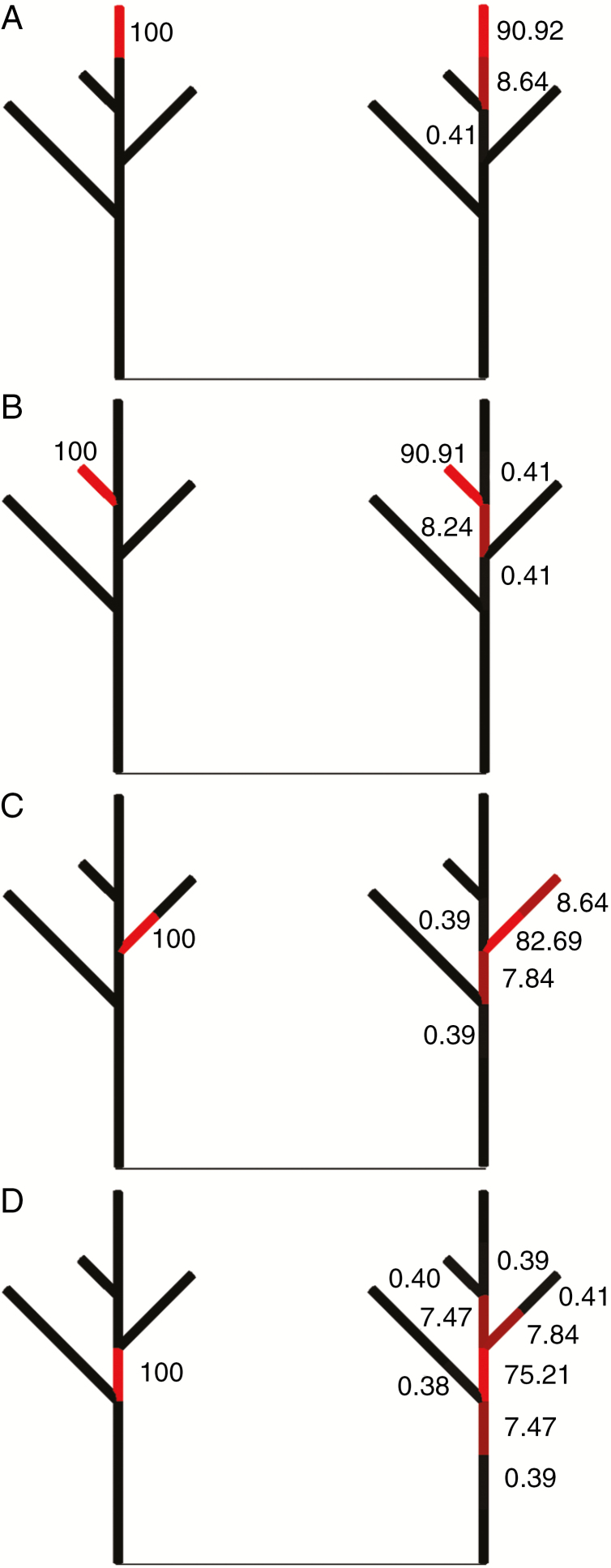
where K_a (d⁻¹) is the transport coefficient, S_n+1 and S_n are the total available carbohydrate from photosynthesis and the local pools at adjacent phytomers n + 1 and n, respectively. A simple example of a static plant structure to illustrate carbohydrate transport with a value for K_a of 0.1 d⁻¹ is shown in Fig. 2.

Fig. 2.

A simple illustration of carbohydrate transport with one step of transport (eqn 6) being solved in a static branching architecture. Panels (A–D) represent the result of carbohydrate transport out of different source internodes, coloured red in the left panels. Phytomers are represented by cylinders, and the shade of red and the value next to the cylinder represent its carbohydrate level. Left panels show the initial distribution of the carbohydrates in the source: at the end of main stem (A), at the end of a branch (B), at the base of a branch (C) and at the middle of the main stem (D). The initial amount of carbohydrate in the source internode was set to 100, and to 0 elsewhere. The panels at the right represent for each initial situation the amount of carbohydrates in each phytomer of the plant after one step transport.

Allocation within a phytomer

After transport, the new amount of carbohydrates for a phytomer either exceeds or subceeds the total potential growth rate of all the organs within this phytomer. In the case of excess these organs reach potential growth and the remaining carbohydrate is stored in the local pool, available for use in the next time step. In the case of insufficiency, organs at the phytomer level receive carbohydrate according to the relative sink strength (Heuvelink, 1996).

$$R_{o,i}=\frac{D_{o,i}}{{{\displaystyle \sum }}_{all organs}{D}_i}$$ (7)

where R_o,i is relative sink strength of organ o (e.g. internode, leaf, fruit) at phytomer i, D_o,i is the absolute sink strength, which is expressed as potential growth rate per day (mg CH₂O organ⁻¹ d⁻¹) calculated from D obtained with eqn (4). ${\displaystyle \sum }_{all organs}{D}_i$ is the total sink strength of all organs at phytomer i. The allocated carbohydrate for growth is converted to dry mass using a factor (R_CM, Table 1) which accounts for growth respiration.

Simulations

For reasons of computational efficiency, simulations were run for small plots of 2 × 2 plants, and these plots were copied ten times in both x and y direction using the replicator functionality of GroIMP to calculate incident radiation on the centre 2 × 2 plants and minimize border effects with respect to the incoming radiation. Simulations were run using the plant population densities and temperature of the field experiment in 2014 (1.5, 7.5 and 13.5 plants m⁻²) to evaluate model performance with respect to biomass production and allocation. The orientation of the first leaf pair was chosen randomly. The dates of sowing and harvesting in simulations were 1 May and 4 October, which is identical to the experiment in 2014. Emergence occurred randomly from 7 to 12 d after sowing (Gu et al., 2014). To obtain plants with realistic fruit retention at the level of the plant, fruit abortion was not mechanistically modelled, but simulated stochastically using observed abscission probabilities at middle square stage and at early boll stage, which resulted in a final rate of boll abortion of ~64 %, similar to experimental observations. Simulation results of the four plants in a plot were averaged. To quantify the heterogeneity of local carbohydrate availability amongst even-aged phytomers, we simulated a cotton plant at a density of 7.5 plants m⁻². This was done without any fruit abortion to avoid disturbance from fruit abscission. The carbohydrate supply was calculated for each phytomer after transport at 100 d after sowing (DAS).

Model validation

The accuracy of model simulations for total leaf area, total above-ground dry mass, dry mass distribution along main stem rank and allocation fractions for each type of organ at the plant level was assessed by comparing simulation results with experimental data collected in 2014. The performance of the model was evaluated using goodness of fit between observed and simulated values, which was expressed as the normalized root mean square error (nRMSE, defined as RMSE divided by the average of the observed values):

$$RMSE=\sqrt{\frac{1}{n}{\displaystyle \sum }_{i=1}^n{\left(X_{sim,i}-X_{obs,i}\right)}^2}$$ (8)

$$nRMSE= \frac{RMSE}{\frac{1}{n}{{\displaystyle \sum }}_{i=1}^n{X}_{obs,i}}$$ (9)

where i is the number of samples, n is the total number of measurements, X_sim,i is the simulated value and X_obs,i is the observed value. The simulations show the best agreement with observations when RMSE and nRMSE are close to 0. The model performance is considered excellent with nRMSE <10 %, good if 10–20 %, acceptable if 20–30 % and poor if >30 % (Jamieson et al., 1991).

To test the ability of the local pool model to represent carbohydrate distribution, we compared the simulated percentage change in the amount of carbohydrate supply for main stem phytomers and for branches at 80 DAS with the measured percentage of total ¹⁴CO₂ detected in different main stem nodes at different ages in the C-labelling experiment of Constable and Rawson (1980a). The percentage change in carbohydrate supply was calculated by dividing the difference between the amount of carbohydrate after and before transport by the amount before transport. A positive percentage represents import, a negative percentage export.

Sensitivity of model output to the transport coefficient

It is difficult to measure the transport coefficient experimentally when simulating carbohydrate transport. To investigate the extent to which the model was sensitive to the value of K_a and was comparable to plant performance in the field, an analysis was performed on the effect of K_a values of 0.01 d⁻¹ (low conductance), 0.02, 0.05, 0.1, 0.5, 1 and 5 d⁻¹ (high conductance) on above-ground biomass and dry mass distribution along the main stem. The parameter value for the transport coefficient cannot be estimated directly from the C-labelling results. Instead, we calibrated the transport coefficient such that the simulated distribution of carbohydrate from main stem leaves was similar to the observed distribution.

RESULTS

Fruiting pattern of cotton

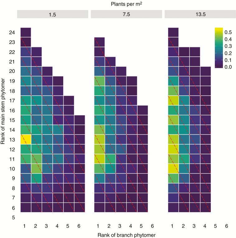
As fruit abscission is closely related to local carbohydrate availability (Guinn, 1982), we analysed variation in carbohydrate availability by checking the measured probability of fruits becoming harvestable (not abscise) in relation to their age class (cohort) (Fig. 3). The number of phytomers potentially bearing a fruit diminished with increasing plant density due to competition. Fruits close to the main stem were the most likely to become harvestable across all densities (light colours in Fig. 3). Fruits that were set further away from the main stem were more prone to abort. Fruits positioned in the lower canopy had a much lower probability of producing a harvestable boll than fruit positions of the same age class in the upper canopy. This analysis of empirical data shows that fruits within a cohort do not have the same probability of becoming harvestable, suggesting that carbohydrate availability is not homogeneously distributed throughout the plant. This supports treating carbohydrate transport in cotton as a process depending on local carbohydrate pools and rejecting a model based on plant-wide homogeneous carbohydrate sharing.

Fig. 3.

Proportion (indicated by colour scale at top right) of nodes at specific main stem and side branch positions having a harvestable boll, measured experimentally in cotton plants at three plant densities: 1.5 (left panel), 7.5 (middle panel) and 13.5 plants m⁻² (right panel). The number on the y-axis indicates the phytomer along the main stem and the number on the x-axis indicates the phytomer along the branch at the corresponding rank of the main stem. Red dashed lines connect phytomers belonging to the same cohort (age class). For nodes of the same age, the probability of boll survival increases with decreasing distance of the fruit from the main stem and increasing main stem rank, suggesting the importance of access to locally produced carbohydrates.

Effect of the transport coefficient

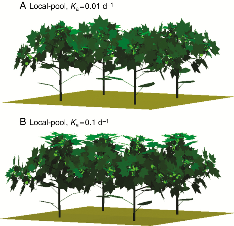
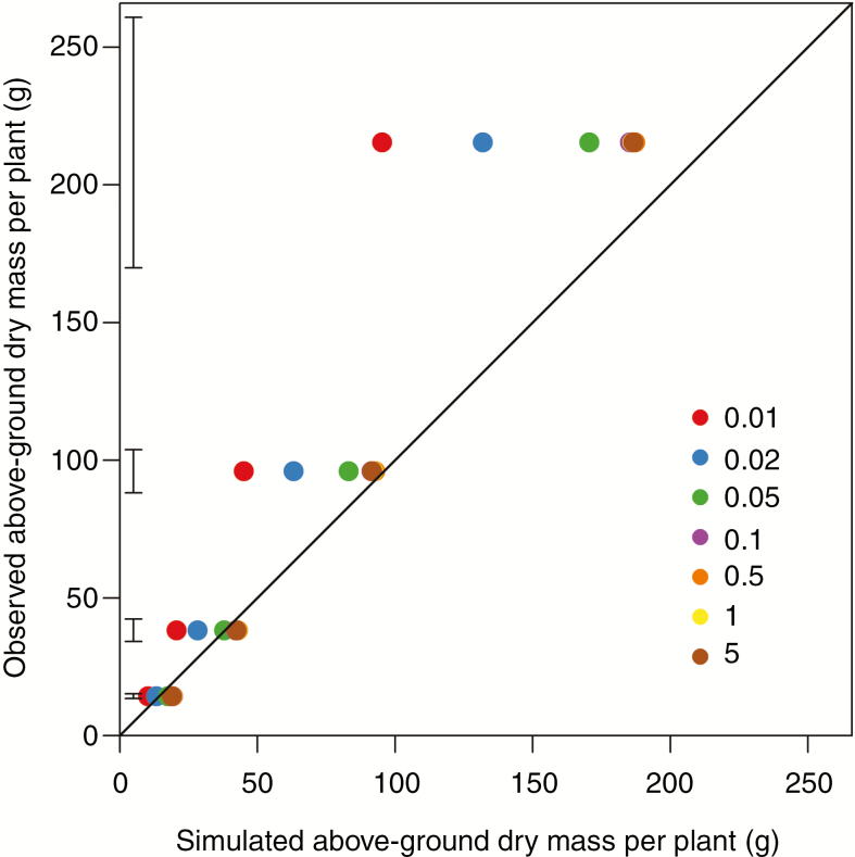
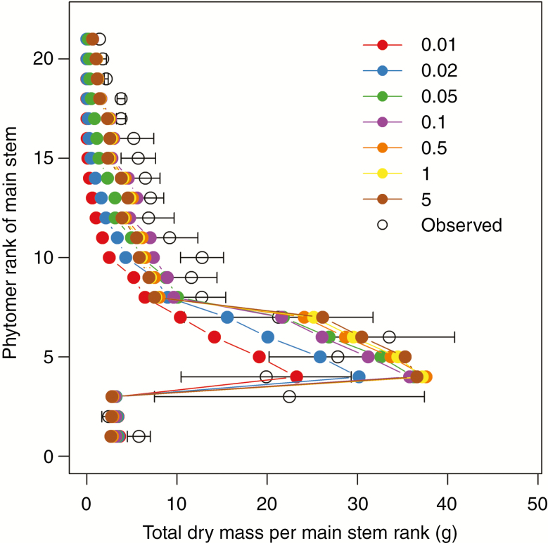
Simulations with a higher transport coefficient K_a resulted in a more vigorous canopy due to the less limiting transport of carbohydrates (Fig. 4A, B). Total above-ground dry mass was substantially underestimated when we used values of K_a <0.1 d⁻¹. Correspondence between observations and simulations was better for larger K_a values up to 0.1 d⁻¹ (nRMSE 72.3, 49.6, 25.6 and 17.0 % for K_a of 0.01, 0.02, 0.05 and 0.1 d⁻¹, respectively). The discrepancy was not reduced further for K_a values beyond 0.1 d⁻¹ (Fig. 5). The dry mass of different main stem phytomers (including the branches at that rank) increased from 2.4 g at lower ranks to a peak of 33.5 g at rank 4 and gradually decreased at higher ranks. This pattern was predicted in simulations for a range of K_a values, but a K_a value of 0.1 d⁻¹ gave the best correspondence (Fig. 6).

Fig. 4.

Visualization of a simulated cotton plot using the local-pool model with transport coefficients of 0.01 (A) and 0.1 d⁻¹ (B) at 90 DAS and a density of 1.5 plants m⁻².

Fig. 5.

Comparison of observed and simulated above-ground dry mass per plant using the local-pool model with transport coefficients of 0.01 (red), 0.02 (blue), 0.05 (green), 0.1 (purple), 0.5 (orange), 1 (yellow) and 5 d⁻¹ (brown) at 53, 62, 74 and 90 DAS at the plant density of 1.5 m⁻² in 2014. Errors bars indicate standard error (n = 4). Note that beyond 0.05 d⁻¹ the symbols overlap and cannot be discriminated individually.

Fig. 6.

Dry mass per main stem phytomer at 90 DAS at a plant density of 1.5 m⁻². Dry mass includes weight of the internode plus the weight of all side branches originating at the internode. Open circles indicate measured values and filled circles connected by solid lines indicate simulated values using a local-pool model with transport coefficients of 0.01 (red), 0.02 (blue), 0.05 (green), 0.1 (purple), 0.5 (orange), 1 (yellow) and 5 d⁻¹ (brown). Error bars indicate standard error of the mean of observations (n = 4).

Effect of density on cotton growth

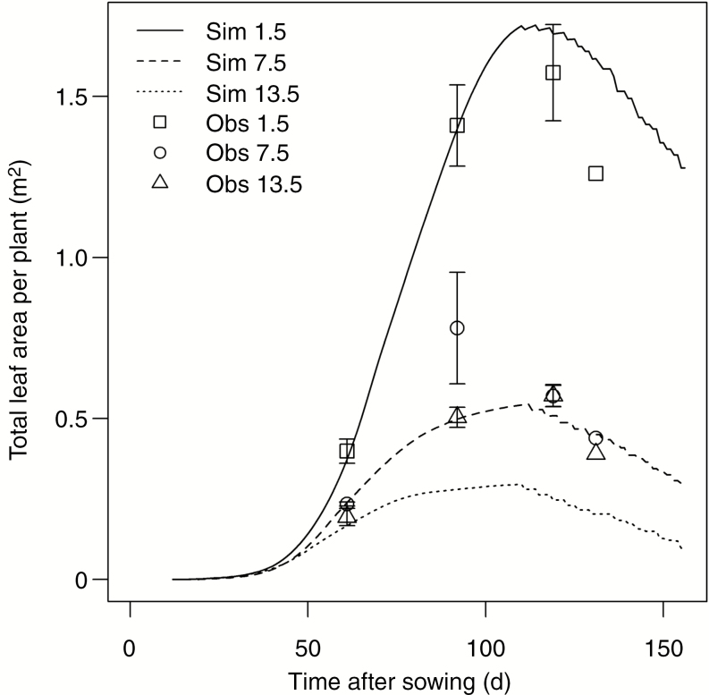
Total leaf area per plant showed a characteristic pattern of expansion and decrease over the growing season at all plant densities (Fig. 7). The leaf area per plant was much higher at lower than at higher densities. At the lowest density, the simulated leaf area agreed well with the observed values from the field, with an nRMSE of 16.2 %. The discrepancy between simulation and observation increased at higher plant densities (nRMSE of 28.6 % at 7.5 plants m⁻² and nRMSE of 52.7 % at 13.5 plants m⁻²).

Fig. 7.

Simulated and observed dynamics of leaf area per plant at plant densities of 1.5, 7.5 and 13.5 m⁻². Lines indicate simulations (Sim), while symbols indicate measurements (Obs). Error bars indicate the standard error of the mean.

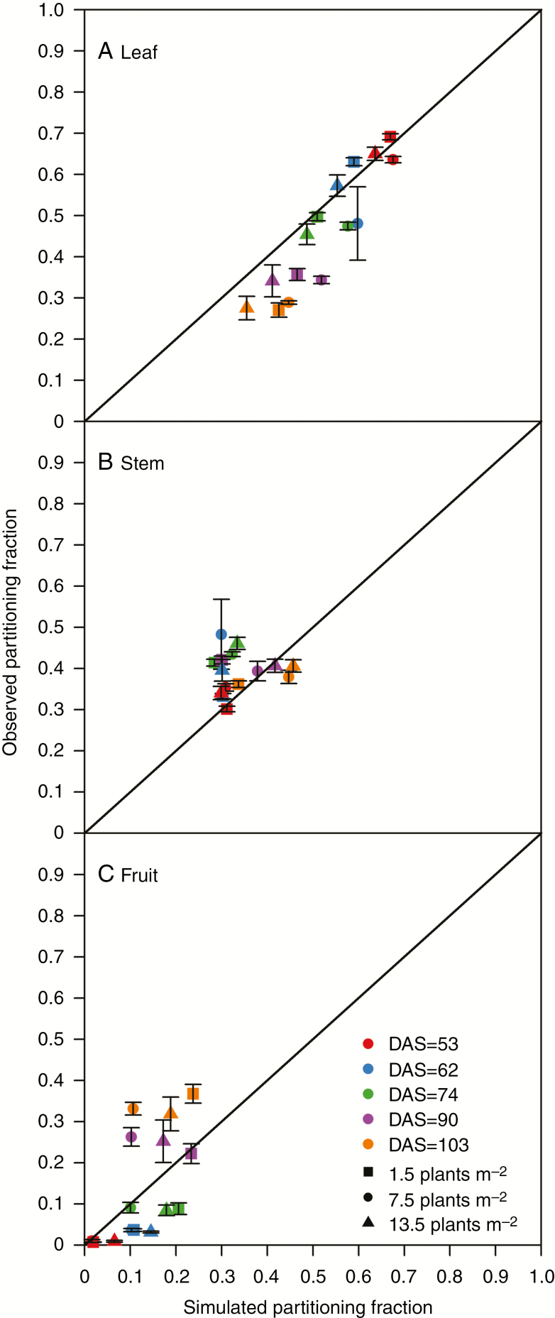
Simulated allocating fractions to leaves (Fig. 8A) and stems (Fig. 8B) showed a good correspondence with observed values across plant densities and growth stages (nRMSE of 20.2 % for leaf and 22.3 % for stem), whereas the allocation to the fruit was underestimated at squaring stage and overestimated at 20 d after flowering (70 DAS in 2014), with an overall nRMSE of 73.3 % caused by the randomized boll shedding within canopy at the same day of 7 d after flowering in the model (Fig. 8C).

Fig. 8.

Simulated allocation fraction to leaf (A), stem (B) and fruit (C) at 1.5 (squares), 7.5 (circles) and 13.5 (triangles) plants m⁻² at 53 (red), 62 (blue), 74 (green), 90 (purple) and 103 (orange) DAS. Error bars indicate the standard error of the mean.

Distribution of carbohydrate

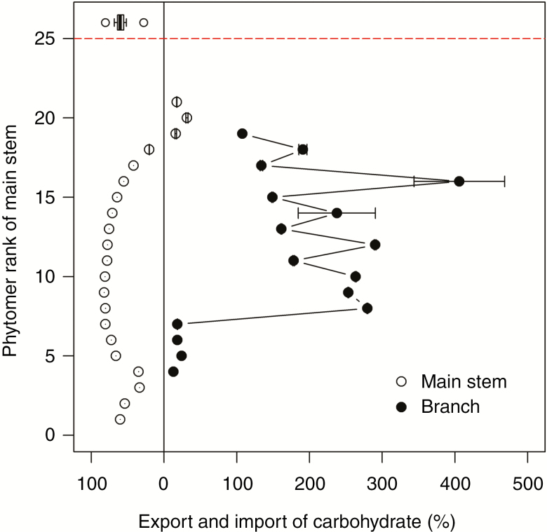
Results on C-labelling from Constable and Rawson (1980a) were used to evaluate the local-pool model. Percentage export of daily local photosynthesis plus storage for most of the main stem phytomers (rank 1 to rank 18) varied from 20 to 80 % irrespective of organ age (Fig. 9) while fruiting phytomers received carbohydrates across the plant, which was in line with the C-labelling results, suggesting that main stem phytomers play a role in exporting carbohydrates to the fruiting branches on the corresponding main stem phytomer and a transport coefficient of 0.1 d⁻¹ is adequate. The variation in percentage import for branches was attributed to the heterogeneity of photosynthesis and local storage due to randomized fruit setting position. The vegetative branches at lower ranks from 4 to 7 imported much less carbohydrate (12–24 %) than fruiting branches because of the carbohydrate production by a great number of leaves on the vegetative branches. Our model captured the budget of carbohydrate for phytomers and predicted translocation of carbohydrate as an emerging result satisfactorily.

Fig. 9.

Simulated percentage export of carbohydrate for main stem phytomers (open circles) and import for branches (black circles with lines) at 80 DAS at the plant density of 4 m⁻² with K_a = 0.1 d⁻¹. Error bars indicate standard error of mean (n = 4) and the measured percentage export of carbohydrate for main stem phytomers (boxplot above the red dashed line) based on the C-labelling dataset from Constable and Rawson (1980a) (branch data not available).

Heterogeneity of local carbohydrate availability

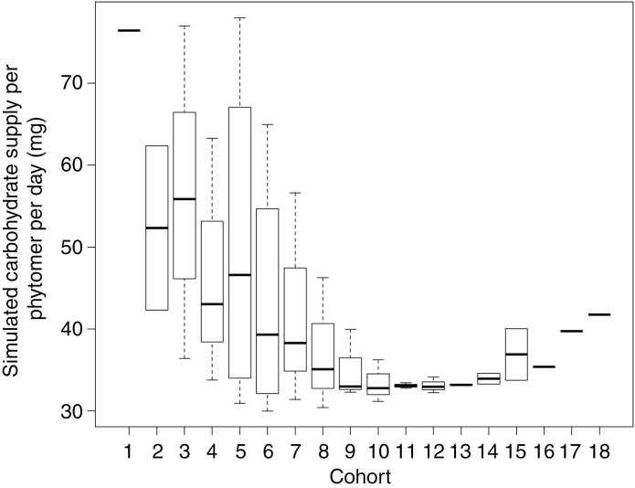
The local-pool model produced a heterogeneous distribution of local carbohydrate availability as an emergent result (Fig. 10). From cohort 10 downwards, phytomers of the same age showed great variation in carbohydrate availability, ranging from 30 to 78 mg CH₂O per phytomer per day. Phytomers in late-season cohorts tended to be more homogeneous in terms of carbohydrate supply than phytomers in early-season cohorts. Phytomers in early-season cohorts had, however, a higher local carbohydrate supply than those in late-season cohorts (Fig. 10). Small variation in carbohydrate supply amongst phytomers in the latest cohorts with the highest main stem rank is at least in part due to a small number of phytomers in these cohorts (e.g. only one value in cohorts 16, 17 and 18).

Fig. 10.

Simulation of daily carbohydrate supply after transport for phytomers at 100 DAS at a plant density of 7.5 m⁻² and K_a = 0.1 d⁻¹. Phytomers in the same cohort share the same x-axis value. The box represents the 25 % and 75 % quartile with a band inside indicating the median. The whiskers represent the maxima and the minima as long as both values are within the 1.5 interquartile-range from the median.

DISCUSSION

Evaluation of model performance

The simulated results in terms of total leaf area per plant, allocating fractions to different organs, above-ground dry mass per plant, and distribution of dry mass along the main stem agree well with experimental measurements in cotton. The new version of CottonXL captures plant performance adequately. However, due to the absence of a mechanistic basis for fruit abortion, which is important in determining carbohydrate transport and thus fruit growth in the current model, we could not yet validate model performance for within-plant boll distribution. A value of 0.1 d⁻¹ for the transport coefficient K_a reproduced empirically observed patterns of transport of carbohydrates from main stem leaves to fruiting phytomers (Fig. 9) (Ashley, 1972; Bhatt, 1976; Constable and Rawson, 1980a). The local-pool model allows the simulation of carbohydrate transport between phytomers within a complex branching architecture and the variability of local carbohydrate availability for phytomers in the same cohort as an emergent result (Fig. 10). The results are qualitatively in line with experimental observations on fruit distribution in the plant (Fig. 3), which is thought to be closely related to local carbohydrate availability (Guinn, 1982).

Underestimation of total leaf area per plant at high densities (Fig. 7) may be due to the absence of shade-avoidance responses in our model, such as reduction in branching, reorientation of leaves, and increased investment in shoot elongation to lift leaves out of the shade (Ballaré and Pierik, 2017; Stewart et al., 2010; Kasperbauer and Hunt, 1992). Such responses may be the reason that real cotton plants performed better at high densities than simulated plants. The allocating fraction to leaves was overestimated (Fig. 8A) after flowering when the allocating fraction to fruits was underestimated (Fig. 8C). The model could be extended with shade-avoidance responses and organ abortion in relation to the imbalance of carbohydrate supply and demand.

Transport of carbohydrate in cotton

Most cotton growth models have been developed based on a global assimilate pool, with the aim of investigating yield formation in relation to cultivar, environment and management (Reddy and Baker, 1988, 1990; Yang et al., 2008). However, our data on the distribution of boll-carrying nodes in the canopy suggest that a global-pool approach is not appropriate for simulating fruit distribution as an emergent model property, just as in many perennial fruit trees (Allen et al., 2005; Cieslak et al., 2011; Pallas et al., 2016). This suggests that the use of a local-pool model in cotton is more appropriate, which is supported by our current modelling results.

To simplify the resistance calculation, we used a fixed value of the transport coefficient or conductance (d⁻¹) for all pathways in a plant. The transport resistance for carbohydrate flow from source to sinks is often estimated by Poiseuille’s law, which states, among other things, that conductance increases quadratically with cross-section area (Sutera and Skalak, 1993). However, the parameter values are difficult to quantify and values may still be far from reality, because resistance will change with temperature and viscosity (Bancal and Soltani, 2002). Our simplification of carbohydrate transport captures the inverse relationship between the proportion of assimilate accumulated by a sink and its distance from the leaf source which was found by Brown (1973). Two considerations support our choice for a simplification of carbohydrate transport using diffusion between phytomers over a global-pool model. First, carbohydrates are transported from endosperm tissue towards the main stem apex instead of towards the root system to sustain shoot growth during the seedling stage, which is in contrast to what a global-pool model predicts (Aoki et al., 2006; Savage et al., 2013). Second, carbohydrates from a leaf cannot be translocated to distant fruits and the amount of transported carbohydrates is inversely related to the distance between source and sink (Ashley, 1972; Bhatt, 1976). Therefore, modelling the transport of carbohydrates via diffusion between phytomers is a plausible approach to the simulation of biomass allocation in cotton.

Calibration of the transport coefficient showed that a higher transport coefficient tended to lead to a better prediction of dry mass, but the discrepancy with experimental data did not diminish any further beyond a K_a value of 0.1 d⁻¹. This indicates that carbohydrates produced by cotton leaves were utilized neither completely locally within a phytomer nor globally across all phytomers within a plant, but were transported to proximate phytomers mostly but not exclusively. In our simulations, carbohydrates were transported from main stem phytomers with high source activity to fruiting phytomers with low source activity, and this is line with a classical series of experiments on sugar movement in cotton plants (Mason and Maskell, 1928a, b).

The chosen modelling approach allowed us to determine the local supply of carbohydrates at the level of the phytomer and predict plant growth as an emerging result. However, there are some limitations in the CottonXL that need to be addressed in the future. First of all, as a compromise between the accuracy and efficiency of computation, FSP models that simulate plant growth based on carbohydrate source/sink dynamics normally run at a model time step of 1 d (Allen et al., 2005) or combine computation for carbohydrate acquisition per day with carbohydrate distribution using smaller time steps (Cieslak et al., 2011). Ideally, simulation of plant carbon economy is done at the same small time step for carbohydrate production, transport and consumption alike. Given the typically stochastic nature of the light models that calculate leaf light absorption (Chelle and Andrieu, 1999; Cieslak et al., 2008), this raises technical issues related to convergence of numerical integration that need to be addressed. Second, although the sink strength was estimated using experimental measurements in a space with minimal plant–plant competition, the organs still competed for finite resources within a plant. This could lead to underestimation of potential maximum dry mass of the organ. Thus, experiments that minimize within-plant competition by defruiting and severe pruning need to be designed in order to more accurately calibrate organ sink strength. Third, experimental measurements will be required to determine the transport coefficient of carbohydrates experimentally instead of through model optimization. It will be necessary to test whether the value is constant over time and across phytomers, not only in cotton but also in other annual crops, like sugarcane (Welbaum et al., 1992) and tomato (Ho, 1996), which utilize carbohydrates locally.

The results presented in this study show that CottonXL, based on local carbohydrate dynamics, is capable of simulating biomass allocation and plant structure, providing support for the hypothesis that assimilate partitioning in cotton is driven not only by sink strength but also by the transport of carbohydrate between phytomers. This work points to a possible use of a local-pool approach to the simulation of fruit distribution, and thus moves cotton eco-physiological modelling forward. To further advance our knowledge of cotton growth, a future step could be to use CottonXL to test the hypothesis that branching pattern (Barbier et al., 2015) and fruit abortion (Gómez-Cadenas et al., 2000) depend on local carbohydrate availability and that fruit loss due to competition could be fully compensated by the increase of individual boll weight (Dai et al., 2015). CottonXL offers a tool for modelling the consequences of local carbon availability, elucidates the mechanism underlying branching and fruit abortion in relation to light environment, and deepens insight into plastic plant responses to density and competition by neighbours.

SUPPLEMENTARY DATA

Supplementary data are available online at www.aob.oxfordjournals.org and consist of the following. Figure S1: frequency of branches at each phytomer rank on main stem in relation to plant densities in 2015. FB and VB indicate fruiting branches and vegetative branches, respectively.

LITERATURE CITED

- Allen MT, Prusinkiewicz P, DeJong TM. 2005. Using L-systems for modeling source–sink interactions, architecture and physiology of growing trees: the L-PEACH model. New Phytologist 166: 869–880. [DOI] [PubMed] [Google Scholar]
- Ashley DA. 1972. C-labelled photosynthate translocation and utilization in cotton plants. Crop Science 12: 69–74. [Google Scholar]
- Aoki N, Scofield GN, Wang X-D, Offler CE, Patrick JW, Furbank RT. 2006. Pathway of sugar transport in germinating wheat seeds. Plant Physiology 141: 1255–1263. [DOI] [PMC free article] [PubMed] [Google Scholar]
- Baker DN, Lambert JR, MacKinion JM. 1983. GOSSYM: a simulator of cotton crop growth and yield. South Carolina Agricultural Experiment Station Technical Bulletin No. 1089. Clemson University, Clemson, SC. [Google Scholar]
- Ballaré CL, Pierik P. 2017. The shade-avoidance syndrome: multiple signals and ecological consequences. Plant, Cell & Environment 40: 2530–2543. [DOI] [PubMed] [Google Scholar]
- Bancal P, Soltani F. 2002. Source–sink partitioning. Do we need Münch?Journal of Experimental Botany 53: 1919–1928. [DOI] [PubMed] [Google Scholar]
- Barbier FF, Lunn JE, Beveridge CA. 2015. Ready, steady, go! A sugar hit starts the race to shoot branching. Current Opinion in Plant Biology 25: 39–45. [DOI] [PubMed] [Google Scholar]
- Berüter J, Droz P. 1991. Studies on locating the signal for fruit abscission in the apple tree. Scientia Horticulturae 46: 201–214. [Google Scholar]
- Bhatt JG. 1976. Translocation of labelled assimilate in morphologically contrasting cotton plants. New Phytologist 76: 53–57. [Google Scholar]
- Brown KJ. 1973. Factors affecting translocation of carbohydrate to fruiting bodies of cotton. Cotton Growing Review 50: 32–42. [Google Scholar]
- Chelle M, Andrieu B. 1999. Radiative models for architectural modelling. Agronomie 19: 225–240. [Google Scholar]
- Cieslak M, Lemieux C, Hanan J, Prusinkiewicz P. 2008. Quasi-Monte Carlo simulation of the light environment of plants. Functional Plant Biology 35: 837–849. [DOI] [PubMed] [Google Scholar]
- Cieslak M, Seleznyova AN, Hanan J. 2011. A functional-structural kiwifruit vine model integrating architecture, carbon dynamics and effects of the environment. Annals of Botany 107: 747–764. [DOI] [PMC free article] [PubMed] [Google Scholar]
- Comtet J, Jensen KH, Turgeon R, Stroock AD, Hosoi AE. 2017. Passive phloem loading and long-distance transport in a synthetic tree-on-a-chip. Nature Plants 3: 17032. doi:10.1038/nplants.2017.32. [DOI] [PubMed] [Google Scholar]
- Constable GA, Rawson HM. 1980a Carbon production and utilization in cotton: inferences from a carbon budget. Australian Journal of Plant Physiology 7: 539–553. [Google Scholar]
- Constable GA, Rawson HM. 1980b Photosynthesis, respiration and transpiration of cotton fruit. Photosynthetica 14: 557–563. [Google Scholar]
- Dai JL, Li WJ, Tang W et al. . 2015. Manipulation of dry matter accumulation and partitioning with plant density in relation to yield stability of cotton under intensive management. Field Crops Research 180: 207–215. [Google Scholar]
- Dauzat J, Clouvel P, Luquet D, Martin P. 2008. Using virtual plants to analyse the light-foraging efficiency of a low-density cotton crop. Annals of Botany 101: 1153–1166. [DOI] [PMC free article] [PubMed] [Google Scholar]
- Dietze MC, Sala A, Carbone MS et al. . 2014. Nonstructural carbon in woody plants. Annual Review of Plant Biology 65: 667–687. [DOI] [PubMed] [Google Scholar]
- Evers JB. 2016. Simulating crop growth and development using functional-structural plant modeling. In: Hikosaka K, Niinemets Ü, Anten PRN, eds. Canopy photosynthesis: from basics to applications. Dordrecht: Springer, 219–236. [Google Scholar]
- Evers JB, Vos J, Chelle M, Andrieu B, Fournier C, Struik PC. 2007. Simulating the effects of localized red:far-red ratio on tillering in spring wheat (Triticum aestivum) using a three-dimensional virtual plant model. New Phytologist 176: 325–336. [DOI] [PubMed] [Google Scholar]
- Evers JB, Vos J, Yin X, Romero P, van der Putten PEL, Struik PC. 2010. Simulation of wheat growth and development based on organ-level photosynthesis and assimilate allocation. Journal of Experimental Botany 61: 2203–2216. [DOI] [PubMed] [Google Scholar]
- Goudriaan J, Van Laar HH. 1994. Modelling potential crop growth processes. Dordrecht: Kluwer. [Google Scholar]
- Génard M. 1992. Effect of leaf number and fruit distribution in peach-trees on the yield and quality of peaches. Canadian Journal of Plant Science 72: 517–525. [Google Scholar]
- Gómez-Cadenas A, Mehouachi J, Tadeo FR, Primo-Millo E, Talon M. 2000. Hormonal regulation of fruitlet abscission induced by carbohydrate shortage in citrus. Planta 210: 636–643. [DOI] [PubMed] [Google Scholar]
- Gould N, Minchin PEH, Thorpe MR. 2004. Direct measurements of sieve element hydrostatic pressure reveal strong regulation after pathway blockage. Functional Plant Biology 31: 987–993. [DOI] [PubMed] [Google Scholar]
- Gu S, Evers JB, Zhang L et al. . 2014. Modelling the structural response of cotton plants to mepiquat chloride and population density. Annals of Botany 114: 877–887. [DOI] [PMC free article] [PubMed] [Google Scholar]
- Guinn G. 1982. Fruit age and changes in abscisic-acid content, ethylene production, and abscission rate of cotton fruits. Plant Physiology 69: 349–352. [DOI] [PMC free article] [PubMed] [Google Scholar]
- Hanan JS, Hearn AB. 2003. Linking physiological and architectural models of cotton. Agricultural Systems 75: 47–77. [Google Scholar]
- Hearn AB. 1994. OZCOT: a simulation model for cotton crop management. Agricultural Systems 44: 257–299. [Google Scholar]
- Hemmerling R, Kniemeyer O, Lanwert D, Kurth W, Buck-Sorlin G. 2008. The rule-based language XL and the modelling environment GroIMP illustrated with simulated tree competition. Functional Plant Biology 35: 739–750. [DOI] [PubMed] [Google Scholar]
- Hemmerling R, Evers JB, Smolenova K, Buck-Sorlin G, Kurth W. 2013. Extension of the GroIMP modelling platform to allow easy specification of differential equations describing biological processes within plant models. Computers and Electronics in Agriculture 92: 1–8. [Google Scholar]
- Heuvelink E. 1996. Dry matter partitioning in tomato: validation of a dynamic simulation model. Annals of Botany 77: 71–80. [Google Scholar]
- Ho L. 1996. The mechanism of assimilate partitioning and carbohydrate compartmentation in fruit in relation to the quality and yield of tomato. Journal of Experimental Botany 47: 1239–1239. [DOI] [PubMed] [Google Scholar]
- Hocking PJ, Steer BT. 1994. The distribution and identity of assimilates in tomato with special reference to stem reserves. Annals of Botany 73: 315–325. [Google Scholar]
- Jamieson PD, Porter JR, Wilson DR. 1991. A test of the computer simulation model ARCWHEAT1 on wheat crops grown in New Zealand. Field Crops Research 27: 337–350. [Google Scholar]
- Kasperbauer MJ, Hunt PG. 1992. Cotton seedling morphogenic responses to FR/R ratio reflected from different colored soils and soil covers. Photochemistry and Photobiology 56: 579–584. [Google Scholar]
- Kniemeyer O. 2008. Design and implementation of a graph grammar based language for functional-structural plant modelling. PhD Thesis, Brandenburg University of Technology, Cottbus, Germany. [Google Scholar]
- Lacointe A. 2000. Carbon allocation among tree organs: a review of basic processes and representation in functional-structural tree models. Annals of Forest Science 57: 521–533. [Google Scholar]
- Mao L, Zhang L, Evers JB et al. . 2016. Identification of plant configurations maximizing radiation capture in relay strip cotton using a functional-structural plant model. Field Crops Research 187: 1–11. [Google Scholar]
- Mason TG, Maskell EJ. 1928a Studies on the transport of carbohydrate in the cotton plant. I. A study of diurnal variation in the carbohydrate of leaf, bark, and wood, and of the effects of ringing. Annals of Botany 42: 189–253. [Google Scholar]
- Mason TG, Maskell EJ. 1928b Studies on the transport of carbohydrate in the cotton plant. II. The factors determining the rate and the direction of movement of sugars. Annals of Botany 42: 571–636. [Google Scholar]
- Mathieu A, Cournede PH, Letort V, Barthélémy D, de Reffye P. 2009. A dynamic model of plant growth with interactions between development and functional mechanisms to study plant structural plasticity related to trophic competition. Annals of Botany 103: 1173–1186. [DOI] [PMC free article] [PubMed] [Google Scholar]
- McDowell NG, Beerling DJ, Breshears DD, Fisher RA, Raffa KF, Stitt M. 2011. The interdependence of mechanisms underlying climate-driven vegetation mortality. Trends in Ecology & Evolution 26: 523–532. [DOI] [PubMed] [Google Scholar]
- McFadyen LM, Robertson D, Sedgley M, Kristiansen P, Olesen T. 2011. Post-pruning shoot growth increases fruit abscission and reduces stem carbohydrates and yield in macadamia. Annals of Botany 107: 993–1001. [DOI] [PMC free article] [PubMed] [Google Scholar]
- Minchin PEH, Lacointe A. 2005. New understanding on phloem physiology and possible consequences for modelling long-distance carbon transport. New Phytologist 166: 771–779. [DOI] [PubMed] [Google Scholar]
- Minchin PEH, Thorpe MR. 2003. Using the short-lived isotope 11C in mechanistic studies of photosynthate transport. Functional Plant Biology 30: 831–841. [DOI] [PubMed] [Google Scholar]
- Niinemets Ü, Anten NPR. 2009. Packing the photosynthetic machinery: from leaf to canopy. In: Laisk A, Nedbal L, Govindjee , eds. Photosynthesis in silico: understanding complexity from molecules to ecosystems. Dordrecht: Springer, 363–399. [Google Scholar]
- Pallas B, Christophe A, Lecoeur J. 2010. Are the common assimilate pool and trophic relationships appropriate for dealing with the observed plasticity of grapevine development?Annals of Botany 105: 233–247. [DOI] [PMC free article] [PubMed] [Google Scholar]
- Pallas B, Da Silva D, Valsesia P et al. . 2016. Simulation of carbon allocation and organ growth variability in apple tree by connecting architectural and source–sink models. Annals of Botany 118: 317–330. [DOI] [PMC free article] [PubMed] [Google Scholar]
- Pan X, Han X, Dong Z. 1997. A cotton growth and development simulation model COTGROW: I. Photosynthesis and dry matter partitioning. Cotton Science 9: 132–141 [in Chinese with English abstract]. [Google Scholar]
- Peuke AD, Rokitta M, Zimmermann U, Schreiber L, Haase A. 2001. Simultaneous measurement of water flow velocity and solute transport in xylem and phloem of adult plants of Ricinus communis over a daily time course by nuclear magnetic resonance spectrometry. Plant, Cell & Environment 24: 491–503. [Google Scholar]
- Piller GJ, Greaves AJ, Meekings JS. 1998. Sensitivity of floral shoot growth, fruit set and early fruit size in Actinidia deliciosa to local carbon supply. Annals of Botany 81: 723–728. [Google Scholar]
- Wickham H. 2009. ggplot2: elegant graphics for data analysis. New York: Springer. [Google Scholar]
- Reddy VR, Baker DN. 1988. Estimation of parameters for the cotton simulation model GOSSYM: cultivar differences. Agricultural Systems 26: 111–122. [Google Scholar]
- Reddy VR, Baker DN. 1990. Application of GOSSYM to analysis of the effects of weather on cotton yields. Agricultural Systems 32: 83–95. [Google Scholar]
- Ritchie GL, Bednarz CW, Jost PH, Brown SM. 2004. Cotton growth and development. Bulletin 1252. Athens, GA: Cooperative Extension Service and the University of Georgia College of Agricultural and Environmental Sciences. [Google Scholar]
- Sadras VO, Bange MP, Milroy SP. 1997. Reproductive allocation of cotton in response to plant and environmental factors. Annals of Botany 80: 75–81. [Google Scholar]
- Savage JA, Zwieniecki MA, Holbrook NM. 2013. Phloem transport velocity varies over time and among vascular bundles during early cucumber seedling development. Plant Physiology 163: 1409–1418. [DOI] [PMC free article] [PubMed] [Google Scholar]
- Savage JA, Clearwater MJ, Haines DF et al. . 2016. Allocation, stress tolerance and carbon transport in plants: how does phloem physiology affect plant ecology?Plant, Cell & Environment 39: 709–725. [DOI] [PubMed] [Google Scholar]
- Stephenson R, Wilson G. 1977. Patterns of assimilate distribution in soybeans at maturity. I. The influence of reproductive development stage and leaf position. Australian Journal of Agricultural Research 28: 203–209. [Google Scholar]
- Stewart SD, Sterling WL. 1988. Dynamics and impact of cotton fruit abscission and survival. Environmental Entomology 17: 629–635. [Google Scholar]
- Stewart JM, Oosterhuis DM, Heitholt JJ, Mauney JR. 2010. Physiology of cotton. Dordrecht: Springer. [Google Scholar]
- Spitters CJT, Toussaint HAJM, Goudriaan J. 1986. Separating the diffuse and direct component of global radiation and its implications for modeling canopy photosynthesis. I. Components of incoming radiation. Agricultural and Forest Meteorology 38: 217–229. [Google Scholar]
- Sutera SP, Skalak R. 1993. The history of Poiseuille’s law. Annual Review of Fluid Mechanics 25: 1–20. [Google Scholar]
- Thornley JHM. 1991. A transport-resistance model of forest growth and partitioning. Annals of Botany 68: 211–226. [Google Scholar]
- Thornley JHM, Johnson IR. 1990. Plant and crop modelling: a mathematical approach to plant and crop physiology. Oxford: Clarendon Press. [Google Scholar]
- Turgeon R. 2010. The role of phloem loading reconsidered. Plant Physiology 152: 1817–1823. [DOI] [PMC free article] [PubMed] [Google Scholar]
- Vos J, Evers JB, Buck-Sorlin GH, Andrieu B, Chelle M, de Visser PHB. 2010. Functional–structural plant modelling: a new versatile tool in crop science. Journal of Experimental Botany 61: 2101–2115. [DOI] [PubMed] [Google Scholar]
- Wang X, Hou Y, Du M et al. . 2016. Effect of planting date and plant density on cotton traits as relating to mechanical harvesting in the Yellow River valley region of China. Field Crops Research 198: 112–121. [Google Scholar]
- Wardlaw IF. 1990. Tansley Review No. 27 – the control of carbon partitioning in plants. New Phytologist 116: 341–381. [DOI] [PubMed] [Google Scholar]
- Watson MA, Casper BB. 1984. Morphogenetic constraints on patterns of carbon distribution in plants. Annual Review of Ecology and Systematics 15: 233–258. [Google Scholar]
- Welbaum GE, Meinzer FC, Grayson RL, Thornham KT. 1992. Evidence for and consequences of a barrier to solute diffusion between the apoplast and vascular bundles in sugarcane stalk tissue. Australian Journal of Plant Physiology 19: 611–623. [Google Scholar]
- Yang Y, Ouyang Z, Yang Y, Liu X. 2008. Simulation of the effect of pruning and topping on cotton growth using COTTON2K model. Field Crops Research 106: 126–137. [Google Scholar]
- Yin X, Goudriaan J, Lantinga EA, Vos J, Spiertz JHJ. 2003. A flexible sigmoid function of determinate growth. Annals of Botany 91: 361–371. [DOI] [PMC free article] [PubMed] [Google Scholar]
- Zhang L, van der Werf W, Cao W, Li B, Pan X, Spiertz JHJ. 2008. Development and validation of SUCROS-Cotton: a potential crop growth simulation model for cotton. NJAS – Wageningen Journal of Life Sciences 56: 59–83. [Google Scholar]
Associated Data
This section collects any data citations, data availability statements, or supplementary materials included in this article.