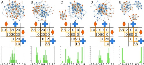
Fig. 2.

Five networks (Top) of $n=40$ nodes and $m=160$ edges with the same global assortativity $r_{\text{global}}=0$, but with different local mixing patterns generated by varying how edges are assigned across subgroups of node types (Middle). The different local mixing patterns can be seen by the distributions of $r_{\text{multi}}$ (Bottom). In A, the mixing pattern is homogeneous across all nodes, and this is reflected in the distribution of $r_{\text{multi}}$ by a unimodal distribution that is peaked around 0. In B–E, there are different heterogeneous mixing patterns, with E being the most extreme case in which half the nodes are highly assortative and half the nodes are highly disassortative. These differences can be observed in the different distributions of $r_{\text{multi}}$.