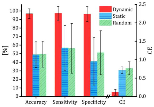
Fig. 2.

Prediction performance, quanitified using accuracy (rate of correct prediction), sensitivity (rate of correct prediction for low-weight loss group), specificity (rate of correct prediction for high-weight loss group) and CE (a measure of prediction error defined as the difference between the prediction grouping probabilities and the real grouping labels, see section 2.7 for detailed definitions) for the dynamic and static connectivity and random grouping analysis. Dynamic connectivity tensors were constructed using a sliding window length of 61 time points and theresholded at connectivity density of 10%. No sliding window was used to make the static netowork; the entire fMRI time series was used to compute a single pairwise correlation matrix for the static networks. For the random grouping analysis, the particpants’ labels were randomly permuted. HOSVD was used to reduce the networks’ rank, HOSVD linearly decomposes the dynamic connectivity tensors to a set of linearly independent (equivalently orthogonal) dynamic connectivity components. To identify the components, HOSVD maximizes the amount of variance captured by the components.