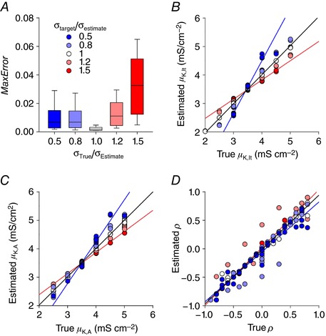
Figure 7. Sensitivity of ion channel density estimation to assumed value of σ.

Sets of spiking pattern proportions were calculated for joint distributions with arbitrarily chosen parameter values. σ_estimate was fixed at 1 mS cm⁻² but, unlike previously fitted distributions, σ_target ( = σ_K,lt and σ_K,A) took a range of values. Specifically, the algorithm was applied to target distributions where σ_estimate correctly estimated σ_target = 1.0 mS cm⁻² (σ_target/σ_estimate = 1.0), σ_target was 20% greater or less than estimated (σ_target/σ_estimate = 1.2 or 0.8, respectively), or σ_target was 50% greater or less than assumed (σ_target/σ_estimate = 1.5 or 0.5, respectively). N = 40 target distributions belonging to each group were used for testing, each with arbitrarily chosen values of μ_K,lt, μ_,K,A and ρ. A, box‐plot shows the MaxError in the estimated spiking pattern proportions, with box ends and whisker ends representing the 1st/3rd quartiles and 5th/95th percentile, respectively. The median error value of 0.002 when σ was correctly estimated (σ_target/σ_estimate = 1.0) was significantly less than when σ was misestimated (P < 0.05, Tukey tests). Estimations of μ_K,lt (B), μ_,K,A (C) and ρ (D) are shown relative to their true values. Black lines show the regression using all points; their slopes were all within 5% of the expected value of 1. However, when the regression was calculated using points from σ_target/σ_estimate = 0.5 (blue) or 1.5 (red), 5 of the 6 values deviated significantly from the expected value of 1 (P > 0.05, one sample t tests with Bonferroni correction).