Figure 2. Sampled conformations from simulations and Markov state models constructed in Q and expected FRET efficiency space.

(A) Scatter plot of sampled conformations from the aggregated trajectories. Representative structures from folded, compact unfolded, and elongated states are shown. Donor and acceptor dyes are colored green and red, respectively. (B) Cluster centers used for constructing the Markov state model are plotted with circles. (C) Initial Markov state model constructed from simulation data only. Node areas are proportional to the equilibrium populations, and edge line widths are proportional to the transition probabilities. (D) Data-assimilated Markov state model after unsupervised learning from smFRET photon-count sequences. Edges with transition probabilities of less than 0.01 are not shown for visual clarity.

Figure 2—figure supplement 1. Q of molecular dynamics simulation trajectories.

(A) Time-course behavior of the fraction of native contacts, Q, is shown for eleven 25.6 μs simulations (starting from unfolded states) and for six 10 μs and four 14 μs simulations (starting from the folded state). All simulations used the force-field of Amber ff99SB. (B) Time-course behavior with a modified Amber ff99SB force-field where the strength between water molecules and protein was scaled. Ten 7 μs simulations (starting from the unfolded states) are shown.

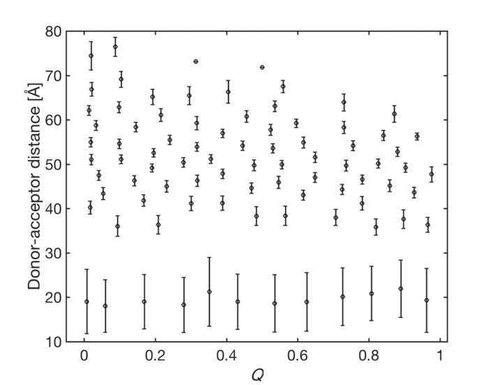
Figure 2—figure supplement 2. Donor-acceptor distances of the Markov states.

The Markov states are plotted in the space spanned by the donor-acceptor distance and Q. Circles represent mean values of two coordinates in the Markov states. The error bar represents the standard deviations of the donor-acceptor distances in the states.

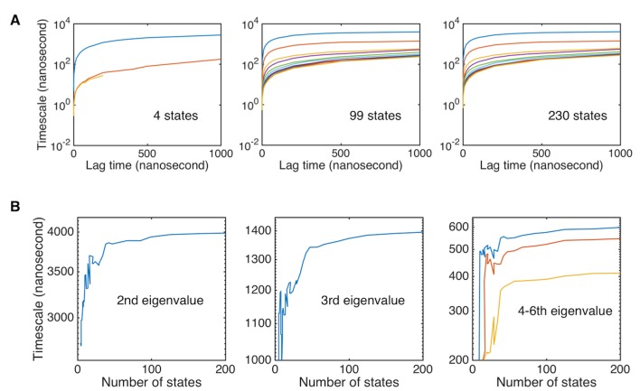
Figure 2—figure supplement 3. Implied timescales for various numbers of states.

(A) Implied timescales for Markov state models built with different numbers of states (4, 99, and 230 states). (B) Converged implied timescales as a function of the number of states. The timescales of the five slowest related to folding dynamics modes are shown.

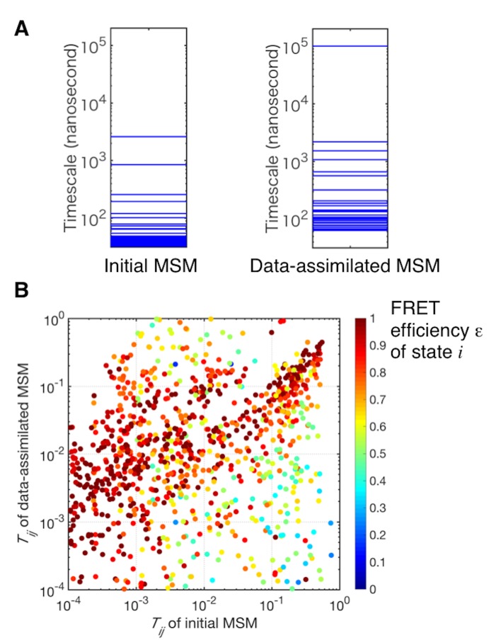
Figure 2—figure supplement 4. Comparison of the transition probabilities of the initial and the data-assimilated Markov state models.

(A) Implied time scales of the initial and the data-assimilated Markov state models. (B) Scatter plot of transition probabilities of the two models. The dots are colored by the FRET efficiencies of the states before transitions (i.e, state i of T_ij).

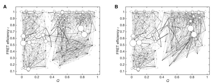
Figure 2—figure supplement 5. Data-assimilated Markov state models using halves of the training data.

(A) Data-assimilated Markov state model obtained using one half set of the single-molecule FRET data. (B) Data-assimilated Markov state model using the other half set. Both models capture similar unfolded, folded, and intermediate states as populated states. Edges with transition probabilities of less than 0.01 are not shown for visual clarity.

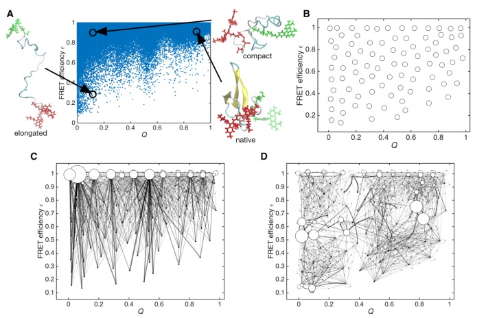
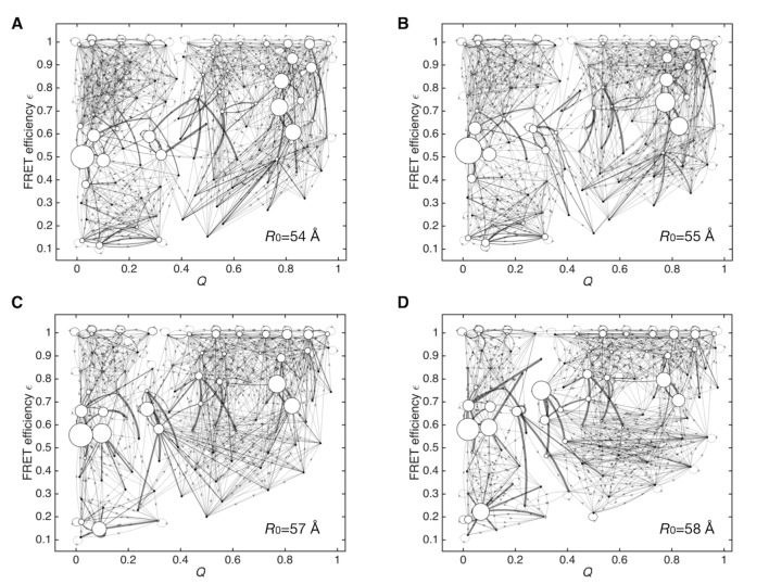
Figure 2—figure supplement 6. Dependency of data-assimilated Markov state models on the choice of Förster radius R₀.

(A) Data-assimilated Markov state model after the convergence of the likelihood function by 10,000 iterations of unsupervised learning using a Förster radius of R₀ = 54 Å. Edges with transition probabilities of less than 0.01 are not shown for visual clarity. (B) R₀ = 55 Å. (C) R₀ = 57 Å. (D) R₀ = 58 Å.

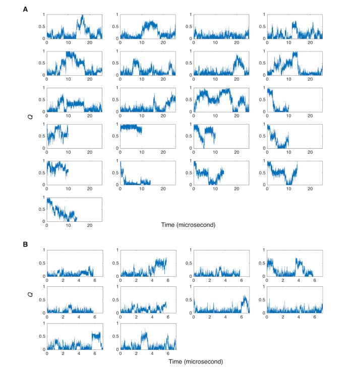
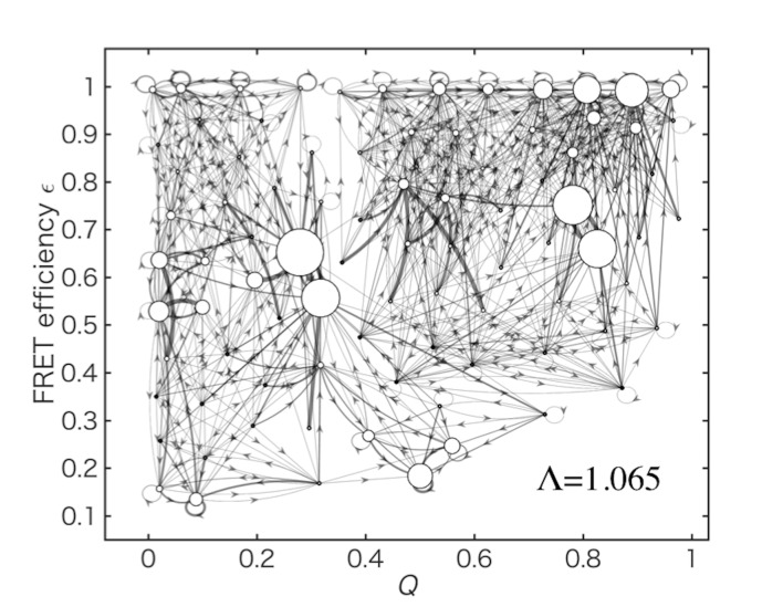
Figure 2—figure supplement 7. Data-assimilated Markov state obtained by considering the FRET efficiency outside the weak-excitation limit.

Data-assimilated Markov state model after the convergence of the likelihood function by 10,000 iterations. Here, a corrected definition of FRET efficiency, which is valid outside the weak-excitation limit (with a parameter $\Lambda =1.065$), was used for the calculation of the likelihood function.

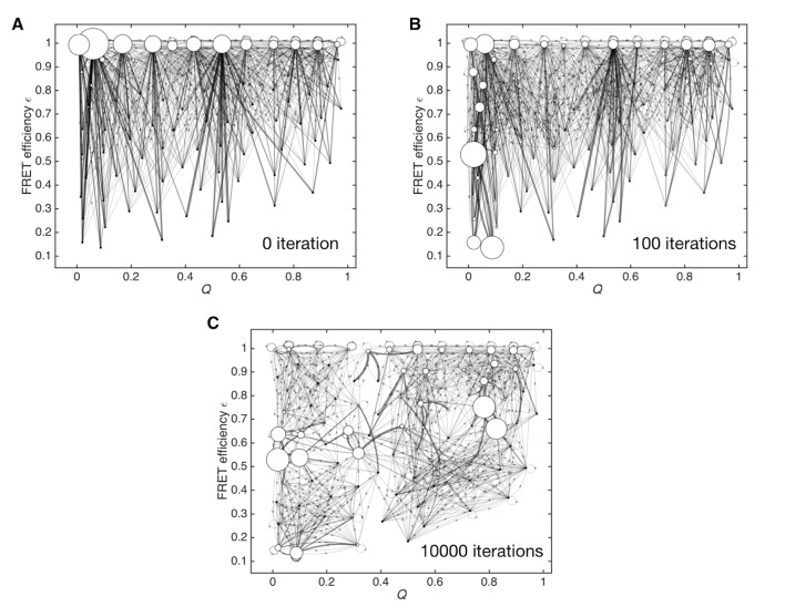
Figure 2—figure supplement 8. Optimization process for the initial Markov state model.

(A) Initial Markov state model constructed only from MD simulation data, used as an initial condition for the unsupervised learning. (B) Markov state model after 100 iterations of unsupervised learning. (C) Data-assimilated Markov state model after the convergence of the likelihood function by 10,000 iterations of unsupervised learning.

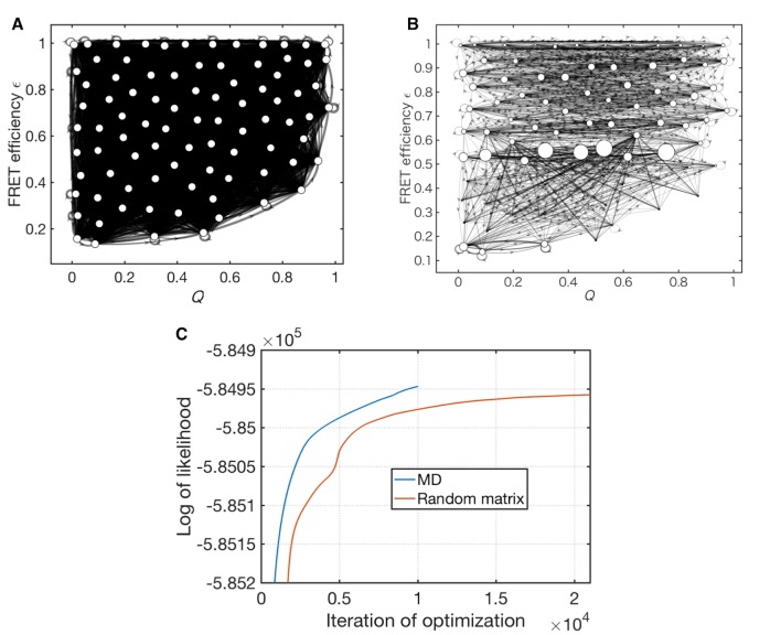
Figure 2—figure supplement 9. Optimization of a random matrix as the initial condition.

(A) Initial Markov state model constructed by assigning random values to the transition probabilities, used as an initial condition for the unsupervised learning. (B) Data-assimilated Markov state model after 21,331 iterations of unsupervised learning. (C) Convergence behavior of the likelihood functions. The blue line corresponds to the initial condition constructed from MD data. The red line indicates the initial condition given from a random matrix.