Comparison of algorithms for the detection of cancer-drivers at sub-gene resolution

Abstract

Understanding genetic events that lead to cancer initiation and progression remains one of the biggest challenges in cancer biology. Traditionally most algorithms for cancer driver identification look for genes that have more mutations than expected from the average background mutation rate. However, there is now a wide variety of methods that look for non-random distribution of mutations within proteins as a signal they have a driving role in cancer. Here we classify and review the progress of such sub-gene resolution algorithms, compare their findings on four distinct cancer datasets from The Cancer Genome Atlas and discuss how predictions from these algorithms can be interpreted in the emerging paradigms that challenge the simple dichotomy between driver and passenger genes.

Introduction

Cancer is a heterogeneous disease that is driven by genomic and epigenomic abnormalities. Recent efforts in cancer genomics have provided us with details of such abnormalities in tens of thousands of human cancers¹. This catalogue has significantly expanded our understanding of the molecular aspects of this disease. However, the mutation landscape, in cancer has turned out to be extremely complex^2-4, as most tumors have hundreds or thousands of somatic mutations, which are seldom found again in other tumors. This apparent heterogeneity is usually interpreted within the driver/passenger paradigm in which the few recurrent mutations are viewed as drivers of the oncogenic process, providing cancer cells with a selective advantage, while most mutations, especially rare ones, are viewed as passengers without any significant consenquences for the cell⁵.

There are many possible ways to identify cancer driver events. For instance, one can look for signals of non-random distribution of mutations at various levels of biological resolution, spanning from individual positions in the protein⁶ up to whole genes⁵ or pathways⁷ (Fig. 1a). Many of the recently developed methods aim to find driver events at the sub-gene level. One advantage of such higher-resolution approaches is that they can identify cases when different mutations in the same gene lead to distinct phenotypes⁸.

Figure 1. Finding mutation drivers across biological scales.

(a) Schematic of different levels for cancer driver detection and the tools used. (b) The four groups of sub-gene resolution algorithms according to the type of regions they find and their number of dimensions. (c) Types of regions detected by each class of algorithm based on EGFR mutations in glioblastoma.

While there are several reviews of cancer driver-detection algorithms^9,10, to the best of our knowledge none has focused on sub-gene resolution algorithms. Given their increasing popularity we decided to review, classify and compare such algorithms and discuss their strengths and weaknesses based on their results on four different cancer datasets. Note that it is not our intention to determine which methods are better, as this is something that likely depends on the type of question being asked, but rather to inform potential users about how the different assumptions and technical choices of each method influence their results. Next, we show how the results of these methods can be integrated with other biological data to gain a deeper understanding of the consequences of mutations in these driver regions. Finally, we discuss the implications that the existence of such mutation clusters might have regarding novel ideas in cancer biology, such as expanding the drivers/passenger paradigm in favor of more nuanced or even continuous models^11-13.

Results

A classification of mutation-clustering algorithms

While the overall goal of all sub-gene resolution driver detection algorithms is the same, identifying non-random clusters of mutations in cancer genomes, the details of their implementations and some of their assumptions can vary significantly. For example, some methods rely solely on the protein sequences^14,15, and therefore can only find clusters of mutations that are linear in the primary sequence. Other methods leverage information from three-dimensional protein structures and can identify spatial patterns that are discontinuous along the sequence^6,16. Similarly, while some algorithms only use the position of the mutations (either in one or three dimensions) to find clusters de novo^16,17, others focus on externally-defined protein regions (such as protein domains^18,19, phosphorylation sites²⁰ or interaction interfaces ^21,22) to identify those enriched in somatic mutations.

Based on these two criteria (number of dimensions and use of externally-defined regions), it is possible to classify sub-gene resolution algorithms into four different groups (Fig 1b,c). In the following paragraphs we list and discuss algorithms from each of these categories. We also provide an overview (further extended in Supplementary Table 1) of their implementation, statistical approaches and their strengths and weaknesses.

Type I – De novo linear clusters

This category includes methods that look for clusters along the gene sequence. The main difference between individual methods from this group is the specific background model they use. While there are methods that rely solely on statistical models^15,23, most of them try to integrate other biological signals such as the distribution of silent mutations^14,24, the ratio between the different types of mutations occurring in a specific gene²⁵, the probability of each mutation given the nucleotide before and after the mutated position^26,27 or by kernel density estimates across multiple biologically relevant scales²⁸.

Type II – De novo three-dimensional clusters

Algorithms that belong to Type II find novel mutation clusters using information about the three-dimensional structure of the protein coded by a given gene. They are more limited in scope that Type I algorithms because they can only be applied to proteins whose three-dimensional structure is either known or can be reasonably predicted. While experimentally determined structures are available only for approximately 6100 human proteins, the structural coverage can be extended to over 13000 proteins²⁹ by aligning proteins to their close homologues with experimental structures (Supplementary Fig. 1).

The biggest differences between Type II algorithms methods are in how they interpret structural data to find mutation clusters. Some tools analyze a re-ordered version of the protein's sequence based on the distance between residues in three dimensions³⁰ or use network algorithms on the graph derived from the structure³¹. However, most Type II algorithms try to identify three-dimensional clusters using the protein structure directly and calculate empirical p-values by re-shuffling the mutations in the structure³². Nevertheless, their specific details can be very different, as some use spheres of varying radii³³, while others use the closeness in the structure-derived residue network⁶, the Shannon entropy of the region¹⁷ or weighted-scoring functions¹⁶. Finally, while most methods can focus solely on individual proteins, others are capable of finding three-dimensional clusters that span across protein complexes¹⁷.

Type III – Linear externally-defined regions

This group contains algorithms that analyze externally-defined linear protein regions to identify those that are enriched in cancer somatic mutations. Therefore, unlike Type I algorithms, these methods can only be applied to proteins where at least one functional region is known, currently limiting their scope to approximately 65% of the human proteome (Supplementary Fig. 1). Such regions can be protein domains¹⁸ or post-translational modification sites²⁰. These algorithms then compare the number of mutations in the selected region with that of the rest of the protein to determine whether there is enrichment in somatic mutations in specific domains or regions. We also include in this category methods that align multiple instances of the same domain in different proteins to find commonly mutated positions^19,34. These methods are based on the rationale that mutations in equivalent positions of the same domain will affect their function in similar ways. These analyses have revealed strikingly similar mutation patterns across domain families such as kinases or the EGF and FGF families of receptors³⁴.

Type IV – Three-dimensional externally-defined regions

Type IV algorithms find three-dimensional externally-defined regions that are enriched in somatic mutations. To the best of our knowledge, this category currently includes only e-Driver3D²¹ and a separate module of CLUMPS¹⁶ (not used here) that uses structurally resolved interaction data¹⁶. This category is most limited in scope, because to be applied it needs to have both structural data and defined functional regions. For example, in the case of e-Driver3D, which currently analyzes protein interaction interfaces, this excludes all proteins that are not involved in structurally resolved complexes. In the case of CLUMPS, the number of proteins and structures that can be analyzed is higher, as it uses information regarding interfaces with DNA, RNA, ion ligands or small molecules in addition to protein partners. However, methods in this category exploit most biological information and, therefore, provide the highest functional information on the mutation clusters they identify.

Methods from the same category tend to identify similar sets of genes

In order to explore the strengths and limitations of each of these four categories, we compared the predictions of methods covering all four categories, as well as two methods that rely on whole-gene analysis^5,35, on four different cancer genomics datasets from The Cancer Genome Atlas¹. We want to stress that the goal of our analysis is not to identify “the best algorithm”, since the classes of methods are complementary. Instead, we aimed to assess how the specific assumptions behind each algorithm affect the number and type of drivers it identifies. We included in our analysis five methods that belong to Type I (Hotspot, NMC¹⁵, OncodriveCLUST¹⁴, MutSig-CL²⁷ and iSIMPRe²³), four from Type II (iPAC³⁰, GraphPAC³¹, SpacePAC³³ and CLUMPS¹⁶), three from Type III (e-Driver¹⁸, ActiveDriver²⁰ and LowMACA¹⁹) and one from Type IV (e-Driver3D³⁶).

Our results (Fig 2a, Supplementary Figs. 2-4 and Supplementary Tables 2-5) show similarities between algorithms that belong to the same category. For example, most Type I, Type II and Type III algorithms tend to cluster together in all datasets. Nevertheless, each group seems to have its own outlier methods. In the case of Type I algorithms, for example, NMC does not cluster with the other methods in the case of BRCA, GBM and LUAD. In the case of Type II algorithms, CLUMPS predictions are very different from those of the family of PAC algorithms in BLCA, BRCA and GBM. Finally, ActiveDriver also seems to identify different genes than the other two Type III algorithms in all datasets. The reasons why these algorithms behave differently from the rest of methods from the same category could be varied. For example, in the case of ActiveDriver it could be because it analyzes post-translational modification sites, unlike the other two Type III algorithms, which focus on protein domains. Therefore, these tools could be finding complementary sets of genes that drive cancer through distinct mechanisms.

Figure 2. Comparison of the overall predictions of each method.

(a) Principal component analysis of the predictions by each method in the four distinct datasets using the p-values for all the genes detected at least by one algorithm. (b) Predictions in the glioblastoma dataset by each method (left panel) and grouped by categories (second panel). Methods are clustered according to the genes they detect. Due to space limitations, we only show genes that are either detected by at least four different algorithms or detected by a single algorithm and that are included in the Cancer Gene Census as missense drivers. We also show the structural coverage of these genes (third panel), whether they are known driver genes (fourth panel) and whether they are oncogenes (OG), tumor suppressor genes (TSG), both (OG/TSG) or known cancer genes whose mode of action still needs to be determined (Unk). Finally, we also show the number of mutations of each gene (right panel).

In terms of specific predictions, most algorithms identify the most frequently mutated cancer driver genes in the different cancer types. For example, all methods identify EGFR and TP53 as GBM driver genes, all but two find PIK3CA and all but three identify IDH1 (Fig. 2b). However, results for other genes exemplify the complementarity between methods from different categories. Again, in the case of GBM, Type II algorithms do not detect PIK3R1 because the missense mutations are spread throughout a large interface. However, Type I, Type III or Type IV algorithms detect the mutation cluster PIK3R1, even that they differ slightly in its exact size and position. In other cases, certain proteins are missed by some methods simply because of lacking statistical power at the selected significance threshold. For example, BRAF, a known driver gene in various cancer types, is also detected as a potential driver in glioblastoma by most sub-gene resolution algorithms but, interestingly, not by the algorithms that work at the gene resolution, OncodriveFM and MutSigCV. A possible explanation for this could be the low mutation frequency of BRAF in this cancer type (8 mutations in 363 samples), making it difficult to detect when comparing its frequency to that of other genes. Nevertheless, 6 of these 8 mutations happen in the residue V600, making it amenable for detection with various sub-gene algorithms. In fact, many genes detected only by sub-gene resolution algorithms, regardless of their category, have relatively low mutation frequencies, when compared to those identified by whole-gene algorithms (Fig. 2b).

Structure-based methods have higher precision but tend to have lower recall than whole-gene approaches

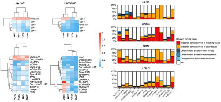
We estimated the precision and recall values for each method and category in each dataset using the list of genes from the Cancer Gene Census (CGC)³⁷ known to play a driver role in each cancer type. The overall results per category show that whole-gene methods have higher recall than any of the sub-gene categories in all four datasets we studied (Fig. 3a). This supports the idea that the whole-gene methods capture classical driver genes. In terms of precision, however, whole-gene methods show similar or lower values than the structure-based algorithms (Types II and IV).

Figure 3. Evaluating the predictions of each method and type of algorithms based on CGC data.

(a) Recall (left) and precision (right) values for each method category in each dataset (top) and each algorithm (bottom). (b) Known driver role of the detected genes by each method according to CGC in each dataset.

As for the individual methods, we observe a clear split in recall values between the two whole-gene methods and any of the sub-gene algorithms, with the former having higher recall values than the latter. In our opinion, there are likely two explanations for this result. The first is that whole-gene algorithms detect both, tumor suppressors and oncogenes, whereas sub-gene algorithms are more likely to detect oncogenes (see below). The second, is that most genes in the gold-standard list have been defined based on their mutation recurrence when compared to the rest of the genome, the signal that whole-gene methods look for. Sub-gene algorithms, however, are designed to detect mutation clusters and take into account only the mutations within a specific gene. While gives an advantage to the sub-gene algorithms in cases of low mutation frequencies (such as BRAF in glioblastoma), it is not how most cancer driver genes have been defined until now. Within sub-gene resolution methods, we observe higher recall values for Type I algorithms than for the rest, probably because, unlike the other categories, they can be applied to any gene. When analyzing the precision data, we found two groups of methods, with CLUMPS, the two e-Driver versions and Hotspot making the group with higher precision values.

Sub-gene resolution methods can find new roles for known cancer genes

Intrigued by the relatively low precision values of most sub-gene resolution algorithms, we classified the genes identified by each method into different categories (Fig. 3b) depending on whether they are known somatic drivers in that specific tissue and whether they are affected by missense mutations or through other genomic alterations (such as copy-number variations or genomic rearrangements). As expected, many of the identified genes are known to be missense somatic drivers in their corresponding tissue. However, there are also 231 genes that are predicted as drivers by at least one method and that, while they do not have any known driver roles in the tissue where they are detected, they are identified as drivers in other tissues. A total of 123 of these genes (53%) are missed by whole-gene methods but, nonetheless, are detected by sub-gene resolution algorithms (Supplementary Table 6).

To our surprise, sub-gene resolution algorithms also detected genes whose driver role is known, but that are usually affected by copy-number variations or genomic rearrangements. For example, PDGFRB acts as a driver in a variety of leukemias via translocations, however, iPAC, GraphPAC, SpacePAC and MutSig-CL all detected it as a potential driver in GBM due to a cluster of mutations in its kinase domain. Similarly, FGFR1 has been linked to breast cancer when amplified, and to myeloproliferative syndromes when translocated. Nevertheless, both ActiveDriver as well as LowMACA, identified a small cluster of mutations in its kinase domain. Another unexpected finding was that several genes known to cause cancer through germline (but not somatic) mutations were identified by some of the methods. The most significant example of this category is CDK4. Germline mutations in this gene are associated with familial melanoma, but 6 sub-gene algorithms identified it as a likely driver in lung adenocarcinoma. Notably, some of the somatic mutations affect the same amino acids as the germline variations associated with melanoma, such as R24L.

Regarding the mode of action of the detected genes, it has been previously suggested that mutation clusters are more frequent in oncogenes, whereas tumor suppressor genes have more distributed mutation patterns¹⁷ (although this notion has been questioned by recent studies¹⁶). Our results support the original observation, as all the sub-gene resolution algorithms, regardless of the type, identify more oncogenes than tumor suppressor genes (Supplementary Fig. 5). In fact, when combining the predictions from all four datasets, there is a statistically significant enrichment of oncogene recognition between 1.4 and 3.7 fold in all sub-gene resolution algorithms (Fisher's test p < 0.01). Whole-gene methods, on the other hand, do not seem to show such bias and detect both tumor suppressor genes as well as oncogenes.

Sub-gene resolution algorithms detect clusters of mutations in novel cancer driver genes

Most sub-gene methods identify non-random mutation distributions in many genes that are not part of the CGC (Fig. 3b). It is likely that some of these genes will be false positives, but many could be true driver genes that are missed by whole-gene methods. Just in the four cancer datasets that we studied there are 66 genes that are not yet known to be somatic drivers and that have been detected by at least three different sub-gene methods but not by the methods that work at the gene resolution (Supplementary Table 7).

Though they are not yet part of the CGC, some of these genes have been reported to have roles in cancer or are likely to have them given their biological functions. For example, OncodriveCLUST, Hostpot and ActiveDriver all detected clusters of mutations in CSNK2A1 in lung adenocarcinoma. This protein is the catalytic subunit of the casein kinase II, a serine/threonine kinase involved in several pathways that are important in cancer, such as Wnt/CTNNB1³⁸ or apoptosis³⁹. Similarly, three algorithms detected a cluster of mutations at in PARP4 in the breast adenocarcinoma dataset (Supplementary Fig. 3). Recent reports suggest that germline mutations in PARP4 might increase the risk to thyroid cancer and breast adenocarcinoma⁴⁰, thus we believe that this gene could play an important role in this type of cancer.

Overall, while one needs to be cautious when interpreting these gene lists and further evidence is needed before the exact role of these genes and mutations in cancer is clear, we believe that sub-gene resolution algorithms can identify valuable potential cancer driver genes missed by approaches that analyze mutation data at other biological scales.

Implications for novel concepts in cancer biology: towards a continuum model of cancer mutations

Only a small number of cancer mutations have well defined and confirmed functional consequences. Most don't and are usually referred to as variants of unknown significance (VUS), as their consequences, in terms of driver effects, are unknown. Many of such VUS are part of mutation clusters recognized as drivers by sub-gene algorithms, which immediately poses the question whether or not these mutations can act as drivers in the patients that carry them. Even that is now possible to systematically test some of these mutations experimentally⁴¹, the most frequent approach to prioritize VUS in cancer driver genes are tools that predict the impact of such mutations in the function of the protein^42,43 or map them into three-dimensional structures^44,45.

Sub-gene resolution algorithms also provide a natural way to predict the impact of these variants and prioritize them. Since most of these methods identify specific clusters of positions within the protein, one can hypothesize that mutations in these positions are the most likely to be carcinogenic, whereas those located in other protein regions are less likely to have any significant driver effect. The power of this classification has been previously exemplified in the analysis of EGFR mutations in glioblastoma. There is a correlation between the location of EGFR mutations in glioblastoma and the overall level of EGFR protein as well as EGFR phosphorylation levels²¹ (Fig. 4a,b,c). Samples with mutations in the dimerization interface have the highest EGFR protein and phosphorylation levels, suggesting a higher activation of the EGFR pathway, while those with mutations in other EGFR regions have an intermediate phenotype between the interface-mutated and the EGFR wild-type samples, a result that has also been recently verified using cancer cell lines⁶. This is consistent with the role of interface and hotspot mutations acting as major-driver events and other EGFR mutations having a different role in cancer. To the best of our knowledge, this phenomenon has not been widely studied and this is one of the few cases analyzed in more detail¹⁶. We believe that sub-gene resolution algorithms will be key to explore such effects.

Figure 4. Using mutation clusters to improve the definition of cancer drivers.

(a) Glioblastoma mutations in EGFR located in the dimerization interface (in red) or in other EGFR positions (yellow). (b) Classification of glioblastoma samples depending on whether they have mutations in the EGFR cluster detected by each method (in red) or other EGFR mutations (in orange). Each row corresponds to a method and each column to a patient. (c) Comparing protein levels measured by RPPA of EGFR (left panel), EGFR pY992 (second panel), EGFR pY1068 (third panel) and EGFR pY1173 (right panel). Samples are classified according to whether they have a mutation in the EGFR-EGFR interface (in red), other EGFR mutations (in orange) or no EGFR mutations (in gray).

Another important point is that the results of these algorithms can also be interpreted as an emerging challenge to the driver/passenger paradigm. Interestingly, conceptual doubts about this paradigm have been formulated for many years. For instance, it was proposed that some drivers may play a role only in specific circumstances, thus being dubbed as latent¹², mini-drivers¹³, or simply part of a continuum of cancer-promoting mutations each with a relatively small but additive effect¹¹. Regardless of the specifics, all these models, at their core, expand on the binary driver/passenger paradigm to go towards a more nuanced classification in which mutations, and the genes they affect, can have different degrees of contribution to cancer growth. The results of sub-gene resolution algorithms provide a natural classification for mutations in well-established cancer driver genes between those that happen in clusters or hotspots (and more likely to be major drivers) and those that happen in other regions of the same protein that are less frequently mutated (more likely to have a lower driver effect or even be passengers). They also identify many genes that are potential low frequency cancer drivers, which could be nevertheless important in specific cases and could lead to actionable predictions as to the molecular mechanism of specific tumors they are found in.

Discussion

We have classified sub-gene resolution driver-detection algorithms into four distinct categorie depending on their overall scope and their data requirements, with each category having a series of advantages and limitations. Overall, these methods find key driver genes in each cancer cohorts, but also identify new genes that are missed by whole-gene approaches. Furthermore, they provide more detailed information than whole-gene approaches, identifying specific protein regions and often suggesting specific mechanisms of driver functions. Integrating the results of these algorithms with other –omic datasets will likely have broad implications for cancer research, including, but not limited to, shedding light into the ongoing efforts to define how mutations contribute to cancer onset and progression.

Also, while we have not explicitly explored this issue, it would likely be possible to apply the same classification (de novo or externally-defined and linear or three-dimensional) to algorithms that detect clusters of non-coding driver mutations. In fact, some of the algorithms discussed here have also been successfully applied to the analysis of non-coding regions²⁶, identifying several mutation clusters in promoters and 5′ UTR among others. Given the relevance of non-coding mutations in cancer⁴⁶, this will be an important issue as whole-genome sequencing becomes more widespread.

Finally, to address the issue of long term sustainability of the benchmarking effort initiated here, we plan to incorporate the methods, input, output and gold standard data sets into the pan-european bioinformatics infrastructure ELIXIR. ELIXIR is currently developing a data warehouse for hosting continuous automated benchmark efforts in this and other areas of life-sciences e.g. homology building in close collaboration with different research communities. Current ELIXIR data warehouse, including documentation and further development plans, is accessible at http://elixir.bsc.es.

Online Methods

Mutation data analysis and pre-processing

We compared the predictions of methods covering all four categories to explore the strengths and limitations of each of them. For Type I we used Hotspot47, NMC15, OncodriveCLUST14, MutSig-CL27 and iSIMPRe23. In the case of Type II we included iPAC30, GraphPAC31, SpacePAC33 and CLUMPS16. As for Type III we included e-Driver^18,21, ActiveDriver20 and LowMACA19. Finally, we used one Type IV algorithm: e-Driver3D^18,21, as well as two methods that rely on whole-gene analysis^5,35.

We analyzed four different cancer genomics datasets from The Cancer Genome Atlas: glioblastoma (GBM, n = 363)⁵⁰, breast adenocarcinoma (BRCA, n = 982)⁵¹, bladder adenocarcinoma (BLCA, n = 137) ⁵² and lung adenocarcinomas (LUAD, n = 546)⁵³. We used Intogen⁵⁴ to predict the location and impact of each mutation in the different protein isoforms from their genomic coordinates (Supplementary Fig. 6). Mutation data come from⁴⁷ instead of the TCGA portal, as it had all the necessary additional information for each mutation in order to run the Hotspot algorithm.

Algorithms

We ran all algorithms using their default settings. In the case of the Hotspot algorithm, we used the genomic information of each mutation provided in the original publication. For Type II methods, when there were multiple three-dimensional structures that could be used as templates to map the mutations, we chose the ones that had the highest structural divergence as defined by PDBFlex⁵⁵. This limits the impact of multiple testing issues and also ensures that we captured proteins that could be affected by protein flexibility. In the case of ActiveDriver, we used all the post-translational modification sites provided with the algorithm: phosphorylations, acetylations and ubiquitinations. For e-Driver and e-Driver3D we used the PFAM domains, disordered regions and protein interfaces described in the original publications.

Evaluation of the results

We used the list of genes included in the Cancer Genome Census³⁷ (downloaded on September 12^th 2016) as benchmark to compare the performance of the algorithms on known driver genes. We limited the list of genes to those that are defined as somatic and that had at least 5 mutations in the dataset being studied. We defined a gene as predicted by an algorithm if its FDR value was below 0.05. The mode of action was also obtained from the CGC list. Note that known cancer genes that are not described as somatic (i.e. only as germline) or as drivers in other tissues in CGC are considered as not known for the purposes of the evaluation.

Regarding the PCA analysis, for each tissue we created a matrix with all the genes detected by at least 2 algorithms and the p-values obtained by each method for each gene. For the purposes of this analysis, all the missing p-values (for example genes with no structures have no p-values for Type II or Type IV algorithms) were assumed to be 1. We calculated the PCA with the minus logarithm of the matrix. The list of candidate novel driver genes identified solely by sub-gene methods was limited only to those genes identified by, at least, three different algorithms. This threshold was defined to minimize the risk of overfitting. This approach that has previously proven useful in detecting cancer driver genes⁵⁶.

EGFR RPPA analysis

We downloaded the normalized glioblastoma RPPA data from the UCSC Cancer Genome Browser⁵⁷ and compared the levels of EGFR-R-C (overall EGFR), EGFR_pY1068-R-V (EGFR phosphorylated at Y1068), EGFR_pY1173-R-C (EGFR phosphorylated at Y1173) and EGFR_pY992-R-V (EGFR phosphorylated at Y992) in three different groups of patients: those with mutations in the EGFR-EGFR interface (based on the PDB coordinates file 3NJP, chains A and B), those with other EGFR mutations and those with no mutations in EGFR. We compared protein expression levels using a two-sided Wilcoxon test.

Data availability

All the algorithms reviewed here can be downloaded from the sites indicated in the Supplementary Table 1. The code and data used to compare the algorithms and generate Figures 2, 3 and 4 can be obtained at: https://github.com/eduardporta/sub-gene_resolution

Table 1. Sub-gene resolution algorithms.

Category	Method	Reference
Type I	OncodriveCLUST	14
	NMC	15
	SomInaClust	25
	Araya et.al.	26
	MutSig-CL	27
	Hotspot	47
	MSEA-Clust	24
	iSIMPRe	23
	M2C	28
Type II	iPAC	30
	GraphPAC	31
	SpacePAC	33
	Hotspot3D	6
	HotMAPS	17
	3DHotspots.org	32
	CLUMPS	16
	mutation3D	48
Type III	ActiveDriver	20
	Yang et.al.	49
	MSEA-Domain	24
	e-Driver	18
	LowMACA*	19
	MutAligner*	34
Type IV	e-Driver3D	21
	CLUMPS	16

^*Both LowMACA and MutAligner analyze all instances of a certain protein domain together, instead of individual protein domains

References

- 1.Cancer Genome Atlas Research, N et al. The Cancer Genome Atlas Pan-Cancer analysis project. Nat Genet. 2013;45:1113–20. doi: 10.1038/ng.2764. [DOI] [PMC free article] [PubMed] [Google Scholar]
- 2.Gerlinger M, et al. Intratumor heterogeneity and branched evolution revealed by multiregion sequencing. N Engl J Med. 2012;366:883–92. doi: 10.1056/NEJMoa1113205. [DOI] [PMC free article] [PubMed] [Google Scholar]
- 3.Watson IR, Takahashi K, Futreal PA, Chin L. Emerging patterns of somatic mutations in cancer. Nat Rev Genet. 2013;14:703–18. doi: 10.1038/nrg3539. [DOI] [PMC free article] [PubMed] [Google Scholar]
- 4.Ortmann CA, et al. Effect of mutation order on myeloproliferative neoplasms. N Engl J Med. 2015;372:601–12. doi: 10.1056/NEJMoa1412098. [DOI] [PMC free article] [PubMed] [Google Scholar]
- 5.Lawrence MS, et al. Mutational heterogeneity in cancer and the search for new cancer-associated genes. Nature. 2013;499:214–8. doi: 10.1038/nature12213. [DOI] [PMC free article] [PubMed] [Google Scholar]
- 6.Niu B, et al. Protein-structure-guided discovery of functional mutations across 19 cancer types. Nat Genet. 2016;48:827–37. doi: 10.1038/ng.3586. [DOI] [PMC free article] [PubMed] [Google Scholar]
- 7.Leiserson MD, et al. Pan-cancer network analysis identifies combinations of rare somatic mutations across pathways and protein complexes. Nat Genet. 2015;47:106–14. doi: 10.1038/ng.3168. [DOI] [PMC free article] [PubMed] [Google Scholar]
- 8.Zhong Q, et al. Edgetic perturbation models of human inherited disorders. Mol Syst Biol. 2009;5:321. doi: 10.1038/msb.2009.80. [DOI] [PMC free article] [PubMed] [Google Scholar]
- 9.Ding L, Wendl MC, McMichael JF, Raphael BJ. Expanding the computational toolbox for mining cancer genomes. Nat Rev Genet. 2014;15:556–70. doi: 10.1038/nrg3767. [DOI] [PMC free article] [PubMed] [Google Scholar]
- 10.Gonzalez-Perez A, et al. Computational approaches to identify functional genetic variants in cancer genomes. Nat Methods. 2013;10:723–9. doi: 10.1038/nmeth.2562. [DOI] [PMC free article] [PubMed] [Google Scholar]
- 11.Leedham S, Tomlinson I. The continuum model of selection in human tumors: general paradigm or niche product? Cancer Res. 2012;72:3131–4. doi: 10.1158/0008-5472.CAN-12-1052. [DOI] [PubMed] [Google Scholar]
- 12.Nussinov R, Tsai CJ. ‘Latent drivers’ expand the cancer mutational landscape. Curr Opin Struct Biol. 2015;32:25–32. doi: 10.1016/j.sbi.2015.01.004. [DOI] [PubMed] [Google Scholar]
- 13.Castro-Giner F, Ratcliffe P, Tomlinson I. The mini-driver model of polygenic cancer evolution. Nat Rev Cancer. 2015;15:680–5. doi: 10.1038/nrc3999. [DOI] [PubMed] [Google Scholar]
- 14.Tamborero D, Gonzalez-Perez A, Lopez-Bigas N. OncodriveCLUST: exploiting the positional clustering of somatic mutations to identify cancer genes. Bioinformatics. 2013;29:2238–44. doi: 10.1093/bioinformatics/btt395. [DOI] [PubMed] [Google Scholar]
- 15.Ye J, Pavlicek A, Lunney EA, Rejto PA, Teng CH. Statistical method on nonrandom clustering with application to somatic mutations in cancer. BMC Bioinformatics. 2010;11:11. doi: 10.1186/1471-2105-11-11. [DOI] [PMC free article] [PubMed] [Google Scholar]
- 16.Kamburov A, et al. Comprehensive assessment of cancer missense mutation clustering in protein structures. Proc Natl Acad Sci U S A. 2015;112:E5486–95. doi: 10.1073/pnas.1516373112. [DOI] [PMC free article] [PubMed] [Google Scholar]
- 17.Tokheim C, et al. Exome-Scale Discovery of Hotspot Mutation Regions in Human Cancer Using 3D Protein Structure. Cancer Res. 2016;76:3719–31. doi: 10.1158/0008-5472.CAN-15-3190. [DOI] [PMC free article] [PubMed] [Google Scholar]
- 18.Porta-Pardo E, Godzik A. e-Driver: a novel method to identify protein regions driving cancer. Bioinformatics. 2014;30:3109–14. doi: 10.1093/bioinformatics/btu499. [DOI] [PMC free article] [PubMed] [Google Scholar]
- 19.Melloni GE, et al. LowMACA: exploiting protein family analysis for the identification of rare driver mutations in cancer. BMC Bioinformatics. 2016;17:80. doi: 10.1186/s12859-016-0935-7. [DOI] [PMC free article] [PubMed] [Google Scholar]
- 20.Reimand J, Bader GD. Systematic analysis of somatic mutations in phosphorylation signaling predicts novel cancer drivers. Mol Syst Biol. 2013;9:637. doi: 10.1038/msb.2012.68. [DOI] [PMC free article] [PubMed] [Google Scholar]
- 21.Porta-Pardo E, Garcia-Alonso L, Hrabe T, Dopazo J, Godzik A. A Pan-Cancer Catalogue of Cancer Driver Protein Interaction Interfaces. PLoS Comput Biol. 2015;11:e1004518. doi: 10.1371/journal.pcbi.1004518. [DOI] [PMC free article] [PubMed] [Google Scholar]
- 22.Vaske CJ, et al. Inference of patient-specific pathway activities from multi-dimensional cancer genomics data using PARADIGM. Bioinformatics. 2010;26:i237–45. doi: 10.1093/bioinformatics/btq182. [DOI] [PMC free article] [PubMed] [Google Scholar]
- 23.Meszaros B, Zeke A, Remenyi A, Simon I, Dosztanyi Z. Systematic analysis of somatic mutations driving cancer: uncovering functional protein regions in disease development. Biol Direct. 2016;11:23. doi: 10.1186/s13062-016-0125-6. [DOI] [PMC free article] [PubMed] [Google Scholar]
- 24.Jia P, et al. MSEA: detection and quantification of mutation hotspots through mutation set enrichment analysis. Genome Biol. 2014;15:489. doi: 10.1186/s13059-014-0489-9. [DOI] [PMC free article] [PubMed] [Google Scholar]
- 25.Van den Eynden J, Fierro AC, Verbeke LP, Marchal K. SomInaClust: detection of cancer genes based on somatic mutation patterns of inactivation and clustering. BMC Bioinformatics. 2015;16:125. doi: 10.1186/s12859-015-0555-7. [DOI] [PMC free article] [PubMed] [Google Scholar]
- 26.Araya CL, et al. Identification of significantly mutated regions across cancer types highlights a rich landscape of functional molecular alterations. Nat Genet. 2016;48:117–25. doi: 10.1038/ng.3471. [DOI] [PMC free article] [PubMed] [Google Scholar]
- 27.Lawrence MS, et al. Discovery and saturation analysis of cancer genes across 21 tumour types. Nature. 2014;505:495–+. doi: 10.1038/nature12912. [DOI] [PMC free article] [PubMed] [Google Scholar]
- 28.Poole W, Leinonen K, Shmulevich I, Knijnenburg TA, Bernard B. Multiscale mutation clustering algorithm identifies pan-cancer mutational clusters associated with pathway-level changes in gene expression. PLoS Comput Biol. 2017;13:e1005347. doi: 10.1371/journal.pcbi.1005347. [DOI] [PMC free article] [PubMed] [Google Scholar]
- 29.Porta-Pardo E, Hrabe T, Godzik A. Cancer3D: understanding cancer mutations through protein structures. Nucleic Acids Res. 2015;43:D968–73. doi: 10.1093/nar/gku1140. [DOI] [PMC free article] [PubMed] [Google Scholar]
- 30.Ryslik GA, Cheng Y, Cheung KH, Modis Y, Zhao H. Utilizing protein structure to identify non-random somatic mutations. BMC Bioinformatics. 2013;14:190. doi: 10.1186/1471-2105-14-190. [DOI] [PMC free article] [PubMed] [Google Scholar]
- 31.Ryslik GA, Cheng Y, Cheung KH, Modis Y, Zhao H. A graph theoretic approach to utilizing protein structure to identify non-random somatic mutations. BMC Bioinformatics. 2014;15:86. doi: 10.1186/1471-2105-15-86. [DOI] [PMC free article] [PubMed] [Google Scholar]
- 32.Gao J, et al. 3D clusters of somatic mutations in cancer reveal numerous rare mutations as functional targets. Genome Med. 2017;9:4. doi: 10.1186/s13073-016-0393-x. [DOI] [PMC free article] [PubMed] [Google Scholar]
- 33.Ryslik GA, et al. A spatial simulation approach to account for protein structure when identifying non-random somatic mutations. BMC Bioinformatics. 2014;15:231. doi: 10.1186/1471-2105-15-231. [DOI] [PMC free article] [PubMed] [Google Scholar]
- 34.Miller ML, et al. Pan-Cancer Analysis of Mutation Hotspots in Protein Domains. Cell Syst. 2015;1:197–209. doi: 10.1016/j.cels.2015.08.014. [DOI] [PMC free article] [PubMed] [Google Scholar]
- 35.Gonzalez-Perez A, Lopez-Bigas N. Functional impact bias reveals cancer drivers. Nucleic Acids Res. 2012;40:e169. doi: 10.1093/nar/gks743. [DOI] [PMC free article] [PubMed] [Google Scholar]
- 36.Porta-Pardo E, Garcia-Alonso L, Hrabe T, Dopazo J, Godzik AA. Pan-Cancer Catalogue of Cancer Driver Protein Interaction Interfaces. PLoS Computational Biology. 2015;11 doi: 10.1371/journal.pcbi.1004518. [DOI] [PMC free article] [PubMed] [Google Scholar]
- 37.Futreal PA, et al. A census of human cancer genes. Nat Rev Cancer. 2004;4:177–83. doi: 10.1038/nrc1299. [DOI] [PMC free article] [PubMed] [Google Scholar]
- 38.Seldin DC, et al. CK2 as a positive regulator of Wnt signalling and tumourigenesis. Mol Cell Biochem. 2005;274:63–7. doi: 10.1007/s11010-005-3078-0. [DOI] [PubMed] [Google Scholar]
- 39.Ahmad KA, Wang G, Unger G, Slaton J, Ahmed K. Protein kinase CK2--a key suppressor of apoptosis. Adv Enzyme Regul. 2008;48:179–87. doi: 10.1016/j.advenzreg.2008.04.002. [DOI] [PMC free article] [PubMed] [Google Scholar]
- 40.Ikeda Y, et al. Germline PARP4 mutations in patients with primary thyroid and breast cancers. Endocr Relat Cancer. 2016;23:171–9. doi: 10.1530/ERC-15-0359. [DOI] [PMC free article] [PubMed] [Google Scholar]
- 41.Brenan L, et al. Phenotypic Characterization of a Comprehensive Set of MAPK1/ERK2 Missense Mutants. Cell Rep. 2016;17:1171–1183. doi: 10.1016/j.celrep.2016.09.061. [DOI] [PMC free article] [PubMed] [Google Scholar]
- 42.Sim NL, et al. SIFT web server: predicting effects of amino acid substitutions on proteins. Nucleic Acids Res. 2012;40:W452–7. doi: 10.1093/nar/gks539. [DOI] [PMC free article] [PubMed] [Google Scholar]
- 43.Creixell P, et al. Kinome-wide decoding of network-attacking mutations rewiring cancer signaling. Cell. 2015;163:202–17. doi: 10.1016/j.cell.2015.08.056. [DOI] [PMC free article] [PubMed] [Google Scholar]
- 44.Mosca R, et al. dSysMap: exploring the edgetic role of disease mutations. Nat Methods. 2015;12:167–8. doi: 10.1038/nmeth.3289. [DOI] [PubMed] [Google Scholar]
- 45.Vazquez M, Valencia A, Pons T. Structure-PPi: a module for the annotation of cancer-related single-nucleotide variants at protein-protein interfaces. Bioinformatics. 2015;31:2397–9. doi: 10.1093/bioinformatics/btv142. [DOI] [PMC free article] [PubMed] [Google Scholar]
- 46.Puente XS, et al. Non-coding recurrent mutations in chronic lymphocytic leukaemia. Nature. 2015;526:519–24. doi: 10.1038/nature14666. [DOI] [PubMed] [Google Scholar]
- 47.Chang MT, et al. Identifying recurrent mutations in cancer reveals widespread lineage diversity and mutational specificity. Nat Biotechnol. 2016;34:155–63. doi: 10.1038/nbt.3391. [DOI] [PMC free article] [PubMed] [Google Scholar]
- 48.Meyer MJ, et al. mutation3D: Cancer Gene Prediction Through Atomic Clustering of Coding Variants in the Structural Proteome. Hum Mutat. 2016;37:447–56. doi: 10.1002/humu.22963. [DOI] [PMC free article] [PubMed] [Google Scholar]
- 49.Yang F, et al. Protein domain-level landscape of cancer-type-specific somatic mutations. PLoS Comput Biol. 2015;11:e1004147. doi: 10.1371/journal.pcbi.1004147. [DOI] [PMC free article] [PubMed] [Google Scholar]
Methods only references
- 50.Brennan CW, et al. The Somatic Genomic Landscape of Glioblastoma. Cell. 2013;155:462–477. doi: 10.1016/j.cell.2013.09.034. [DOI] [PMC free article] [PubMed] [Google Scholar]
- 51.Koboldt DC, et al. Comprehensive molecular portraits of human breast tumours. Nature. 2012;490:61–70. doi: 10.1038/nature11412. [DOI] [PMC free article] [PubMed] [Google Scholar]
- 52.Weinstein JN, et al. Comprehensive molecular characterization of urothelial bladder carcinoma. Nature. 2014;507:315–322. doi: 10.1038/nature12965. [DOI] [PMC free article] [PubMed] [Google Scholar]
- 53.Collisson EA, et al. Comprehensive molecular profiling of lung adenocarcinoma. Nature. 2014;511:543–550. doi: 10.1038/nature13385. [DOI] [PMC free article] [PubMed] [Google Scholar]
- 54.Gonzalez-Perez A, et al. IntOGen-mutations identifies cancer drivers across tumor types. Nat Methods. 2013;10:1081–2. doi: 10.1038/nmeth.2642. [DOI] [PMC free article] [PubMed] [Google Scholar]
- 55.Hrabe T, et al. PDBFlex: exploring flexibility in protein structures. Nucleic Acids Res. 2016;44:D423–8. doi: 10.1093/nar/gkv1316. [DOI] [PMC free article] [PubMed] [Google Scholar]
- 56.Tamborero D, et al. Comprehensive identification of mutational cancer driver genes across 12 tumor types. Sci Rep. 2013;3:2650. doi: 10.1038/srep02650. [DOI] [PMC free article] [PubMed] [Google Scholar]
- 57.Goldman M, et al. The UCSC Cancer Genomics Browser: update 2015. Nucleic Acids Res. 2015;43:D812–7. doi: 10.1093/nar/gku1073. [DOI] [PMC free article] [PubMed] [Google Scholar]
Associated Data
This section collects any data citations, data availability statements, or supplementary materials included in this article.
Supplementary Materials
Supplementary Figure 1. Coverage of the human proteome by different types of biological features
Fraction of the proteome that is covered by linear regions (left), structures with over 95% sequence identity between the protein and the template (middle) or structures with a BLAST e-value between the protein and the template below 1e-9. The fraction is calculated for both, the absolute number of proteins (left columns) as well as the total number of residues (right columns). The distinction between the two is important because it is usually the case that we only know the structure for a fraction of the protein.
Supplementary Figure 2. Results of the different algorithms in the BLCA dataset.
Visualization is limited to genes detected by at least 4 methods or known drivers in BLCA detected by at least one algorithm.
Supplementary Figure 3. Results of the different algorithms in the BRCA dataset.
Visualization is limited to genes detected by at least 4 methods or known drivers in BRCA detected by at least one algorithm.
Supplementary Figure 4. Results of the different algorithms in the LUAD dataset.
Visualization is limited to genes detected by at least 4 methods or known drivers in LUAD detected by at least one algorithm.
Supplementary Figure 5. Sub-gene resolution algorithms detect more oncogenes than tumor-suppressors
(a) Barplot showing the fraction of genes detected by each method that are oncogenes, tumor-suppressors, have a dual-role or whose mode of action is not yet known. (b) Fold-enrichment of each method in detected oncogenes or genes with dual-role when aggregating all four datasets.
Supplementary Figure 6. Description of the datasets.
(a) Mutation types in each patient of the different dataset. The majority of mutations are missense. (b) Number of patients (top) and violin plot showing the distribution of number of mutations (bottom) in each dataset. Each dot represents a sample.
Data Availability Statement