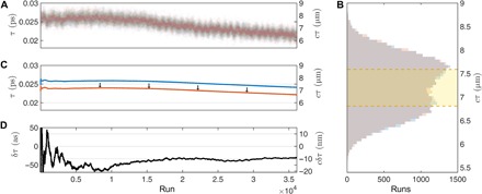
Fig. 3. Example of an acquired experimental data set.

(A) Individual estimates of τⁱⁿ (blue) and τ^out (red) for two piezo positions separated by 10 nm (33.3 as). A relatively large drift can be seen in the data, which is dealt with by switching between piezo positions as discussed above. (B) The histogram shows two almost perfectly overlapping distributions. Classical interferometry would be limited to a distribution no larger than the yellow area. The distributions are generally nonunimodal, which is indicative of significant drift (or slowly varying noise). (C) Cumulative estimates are plotted. The drift in each estimate is considerable, being approximately 2 fs (600 nm). The red curve has been shifted down by 2 fs for clarity (arrows). The drift for each sample position is very well correlated because we switch the sample position much faster than the drift. (D) Because of this correlation, the difference in cumulative estimates δτ is very stable and converges on the true value.