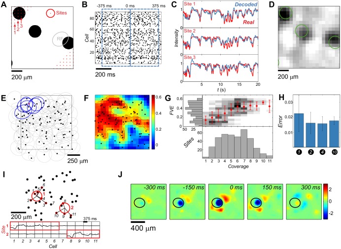
Fig 1. Linear decoding of a complex movie.

A: An example stimulus frame. At each site (red dots = partially shown 20×20 grid) the stimulus was convolved with a spatial gaussian filter (red circle = 1σ). Typical RGC receptive field center size shown in gray. B: Responses of 91 RGCs with 750 ms decoding window overlaid in blue. C: Three example luminance traces (red) and the linear decoders’ predictions (blue). D: Decoded frame (same as in A) reconstructed from 20×20 separately decoded traces. Disc contours of the original frame shown for reference in green. E: RF centers of the 91 cells (black dots = centers of fitted ellipses). RF centers overlapping a chosen site (red dot) are highlighted in blue. F: Performance of the linear decoders across space, as Fraction of Variance Explained (FVE). Black dots as in E; black contour is the boundary FVE = 0.4. G: Performance of the linear decoders (FVE) across sites as a function of cell coverage (grayscale = conditional histograms, red dots = means, error bars = ± SD). H: Average decoding error across sites (MSE ± SD) of 10-disc-trained decoders, tested on withheld stimuli with different numbers of discs. I: Cells (black dots = RF center positions) contributing to the decoding at two example sites (red circles); decoding filters shown below. For each site, contributing cells (highlighted in red and joined to the site) account for at least half of the total L1 norm. J: Decoding field of a single cell (here, evaluated over a denser 50×50 grid and normalized to unit maximal variance); the cell’s RF center shown in black.