LeNup: learning nucleosome positioning from DNA sequences with improved convolutional neural networks

Abstract

Motivation

Nucleosome positioning plays significant roles in proper genome packing and its accessibility to execute transcription regulation. Despite a multitude of nucleosome positioning resources available on line including experimental datasets of genome-wide nucleosome occupancy profiles and computational tools to the analysis on these data, the complex language of eukaryotic Nucleosome positioning remains incompletely understood.

Results

Here, we address this challenge using an approach based on a state-of-the-art machine learning method. We present a novel convolutional neural network (CNN) to understand nucleosome positioning. We combined Inception-like networks with a gating mechanism for the response of multiple patterns and long term association in DNA sequences. We developed the open-source package LeNup based on the CNN to predict nucleosome positioning in Homo sapiens, Caenorhabditis elegans, Drosophila melanogaster as well as Saccharomyces cerevisiae genomes. We trained LeNup on four benchmark datasets. LeNup achieved greater predictive accuracy than previously published methods.

Availability and implementation

LeNup is freely available as Python and Lua script source code under a BSD style license from https://github.com/biomedBit/LeNup.

Supplementary information

Supplementary data are available at Bioinformatics online.

1 Introduction

Nucleosome positioning broadly indicates where nucleosomes are located with respect to the genomic DNA sequence (Struhl and Segal, 2013). Composed of DNA and a protein core, nucleosomes are about 10 nm in diameter and are the fundamental repeating unit of chromatin structure of eukaryotic DNA (Kornberg and Lorch, 1999; Richmond and Davey, 2003). The core is an octamer containing two copies each of histones H2A, H2B, H3 and H4. The histone octamer forms a wedge-shaped disk, around which 147 base pairs of DNA are tightly wrapped in approximately 1.7 turns in a left-handed superhelix (Luger et al., 1997). The DNA segment connecting two adjacent nucleosomes is referred to as a linker. Nucleosome positioning is critical to various biological processes, primarily because this precise positioning modulates the accessibility of underlying genomic sequence to DNA-binding proteins to regulate transcription (Liu M. et al., 2015; Schones et al., 2008; Tilgner et al., 2009; Whitehouse et al., 2007), genetic replication (Eaton et al., 2010; Liu et al., 2017; Vasseur et al., 2016), and recombination (Pulivarthy, 2016; Smagulova et al., 2011). Therefore, the identification of nucleosome positioning along genomic sequences may allow an in-depth understanding of various biological outcomes. Although many studies provide for support that the genome-wide pattern of nucleosome positioning is associated with DNA sequence, nucleosome remodelers and transcription factors including activators, components of the preinitiation complex and elongating Pol II (Segal and Widom, 2009; Struhl and Segal, 2013), the determinant factors of the nucleosome positioning are still far from a quantitative understanding. The intrinsic DNA sequence preferences of nucleosomes may be a dominant role in the nucleosome organization (Kaplan et al., 2009). Early discoveries indicate that distinctive sequence motifs play an important role in nucleosome positioning. Part of these discoveries include 10-bp interval repetition of AA/TT/TA dinucleotides (Ioshikhes et al., 1996; Satchwell et al., 1986), and TATAAACGCC repeat sequence (Widlund et al., 1999). Some research results establish that nucleosome organization is encoded in eukaryotic genomes and that this intrinsic organization can explain approximately 50% of the in vivo nucleosome positions (Segal et al., 2006). Another work claimed that about 75% of nucleosomes are characterized by sequences (Ioshikhes et al., 2011).

In the last decade, high-throughput genome-wide data with respect to nucleosome positioning come from a number of related techniques, such as MNase-seq (Jiang and Pugh, 2009; Kaplan et al., 2009; Weiner et al., 2009), DNase-seq (Bell et al., 2011; Guertin and Lis, 2013; Liu et al., 2016; Zhong et al., 2016) and ChIP-seq (Schones et al., 2008). These techniques have an idea in common to cut DNA between nucleosomes and map protected DNA regions. High-resolution genome-wide nucleosome maps were obtained for several organisms including yeast (Brogaard et al., 2012; Lee et al., 2007; Yuan et al., 2005), drosophila (Mavrich et al., 2008a), Caenorhabditis elegans (Valouev et al., 2008) and human (Barski et al., 2007; Schones et al., 2008; Valouev et al., 2011). The high-resolution data have been deeply promoting the development of computational methods for accurately predicting nucleosome positioning (Awazu, 2017; Chen et al., 2012; Guo et al., 2014; Gupta et al., 2008; Morozov et al., 2009; Segal et al., 2006; Van der Heijden et al., 2012; Wang et al., 2012; Xi et al., 2010).

Assuming that each 147-bp sequence in favor of histone-DNA interaction is a Markov chain, Segal et al. proposed a probabilistic model (Segal et al., 2006) to predict genome-wide nucleosome positioning in yeast. The model was improved by incorporating the information of linker sequences (Field et al., 2008). N-score (Yuan and Liu, 2008) distinguished nucleosomal sequences from non-nucleosome sequences adopting a wavelet analysis based model and a logistic regression model for predicting nucleosome positions from DNA sequence. NuPoP (Xi et al., 2010) models the DNA sequence with a duration hidden Markov model of two alternative states: nucleosome (N) and linker (L). A fourth order time-dependent Markov chain was trained for the N state, and a homogeneous fourth-order Markov chain for the L state. NuPoP outputs nucleosome occupancy score and nucleosome affinity score. Stimulated by the PseAAC approach (Chou, 2001; Chou, 2005), a sequence-based predictor called iNuc-PseKNC (Guo et al., 2014) for nucleosome positioning in genomes with pseudo k-tuple nucleotide composition was proposed. Here, the samples of DNA sequences were formulated using six basic DNA local structural properties and a support vector machine (SVM) classifier was trained on datasets from H. sapiens, C. elegans and Drosophila melanogaster. It was shown that iNuc-PseKNC had better performance in the prediction of nucleosome positioning than previously developed predictors. Furthermore, using the similar methodology to iNuc-PseKNC, more recently improved models (Awazu, 2017; Chen et al., 2016) were developed for the prediction of nucleosome positioning.

The computational methods and tools promoted and advanced the understanding on nucleosome positioning. However, most of these algorithms deeply depend on either the recognition of distribution of the nucleotides in nucleosome sequences (Awazu, 2017; Guo et al., 2014; Segal et al., 2006; Van der Heijden et al., 2012; Wang et al., 2012; Xi et al., 2010) or the measurement of biophysical and(or) physicochemical properties (Chen et al., 2012; Minary and Levitt, 2014). As Nucleosome positioning is strongly affected by DNA sequence (Gonzalez, 2016; Miele et al., 2008; Segal and Widom, 2009; Struhl and Segal, 2013; Zhang et al., 2009), computers may automatically learn the representation of Nucleosome positioning from the DNA sequences. This idea can be achieved by deep learning (Hinton and Salakhutdinov, 2006; Kelley et al., 2016; LeCun et al., 2015; Leung et al., 2014) that allows computational models to learn representations of data (Bengio et al., 2013) from multiple levels of abstraction. Deep learning has produced extremely promising results in image recognition (Krizhevsky et al., 2012), speech recognition (Hinton et al., 2012), natural language understanding (Collobert et al., 2011a), genetic variants scoring (Xiong et al., 2015), Go play (Silver et al., 2016) and cancer classification (Esteva et al., 2017).

In this study, a novel nucleosome positioning predictor was developed based on the convolutional neural networks (CNN). We set up a rigorous intellectual deep-learning network mainly composed by GoogleNet Inception convolutional neural network architecture (Szegedy et al., 2016) and gated convolutional networks (Dauphin et al., 2016). After training, the performance of the system was measured on a different set of examples called a test set. This predictor exhibited more excellent performance than the recently developed predictors for the same benchmark datasets of human, worm, fly and yeast genomes.

2 Materials and methods

To learn nucleosome positioning, we introduce a new deep convolutional architecture which is composed by the Inception deep convolutional architecture (Szegedy et al., 2015) and gated convolutional networks (Dauphin et al., 2016). Gated convolutional networks (Dauphin et al., 2016) were originally introduced for language modeling which outperformed strong recurrent models on language modeling.

2.1 Benchmark datasets of nucleosome positioning and nucleosome-disfavoring sequences

The benchmark datasets of nucleosome positioning and nucleosome-disfavoring sequences were downloaded from the Supplementary Material of two published papers (Chen et al., 2016; Guo et al., 2014). These datasets involve H. sapiens, C. elegans, D. melanogaster (Guo et al., 2014) and Saccharomyces cerevisiae (Chen et al., 2016). Only the low-biased benchmark datasets were used to train and test LeNup in this study.

2.2 Principle of a deep learning network for one-dimensional sequences

In a deep learning network, one processing step is usually called a layer, which could be a convolution layer, a ReLU layer, a pooling layer, a dropout layer, a normalization layer, a fully connected layer, a loss layer, etc. Unlike the three-dimensional feature tensor of an image, a one-dimensional DNA sequence has only a two-dimensional feature matrix. The width and depth of the matrix correspond with the number of row and column of the feature matrix. There is no height of a 2D matrix, but we say that the height is equal to 1 to be consistent with 3D feature tensors. Figure 1 illustrates the process of multiple convolutions, ReLU and pooling to the sequence feature matrix. Suppose we are considering the l–th layer, whose inputs form a two-dimensional feature matrix ${\mathbf{X}}^l$ with ${\mathbf{X}}^l\in {ℝ}^{m\times N}$. Assuming D filters are used and each filter is of spatial span m × k (for instance, k = 3), we pad the feature matrix by adding $\frac{k}{2}$ columns with all elements being zero to the head and tail of the matrix. Therefore, the width of new features after convolutional operation with stride 1 is still N. The rectified linear unit (ReLU) f(z) = max(0, z) is applied in the networks. Pooling operations where every two adjacent elements are merged into one element. As shown in Figure 1, the outputs form the two-dimensional feature matrix ${\mathbf{X}}^{l+1}$ with ${\mathbf{X}}^{l+1}\in {ℝ}^{D\times \frac{N}{2}}$.

Fig. 1.

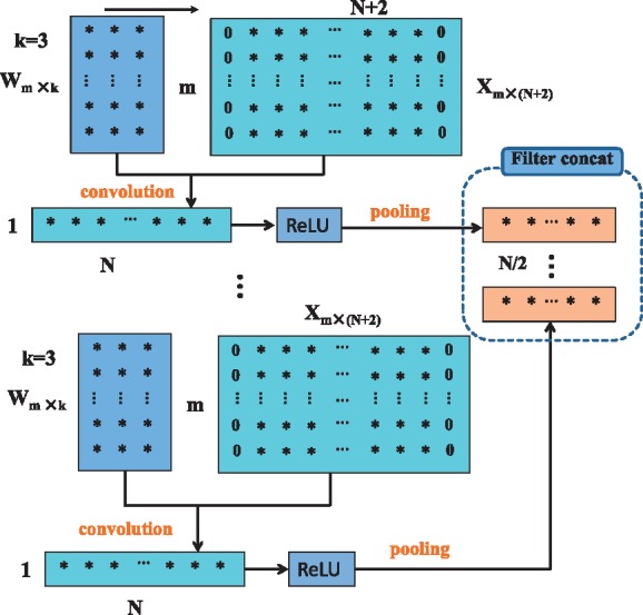
The schema of convolution, ReLU and pooling in a deep learning network for one-dimensional sequence

2.3 Inception networks

Starting in 2014, the quality of network architectures significantly improved by utilizing deeper and wider networks. The Inception architecture of GoogLeNet (Szegedy et al., 2015) performed well even under strict constraints on memory and computational budget. The Inception models used to be trained in a partitioned manner, where each replica was partitioned into a multiple sub-networks in order to be able to fit the whole model in memory (Szegedy et al., 2016). A practically useful aspect of the Inception-style networks is that it aligns with the intuition that nucleosome positioning information should be processed at various scales and then be aggregated so that the next stage can abstract features from different scales simultaneously. Figure 2 shows the original Inception model (Szegedy et al., 2015) in visual recognition.

Fig. 2.

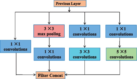
Original Inception module for classification and detection in the ImageNet Large-Scale Visual Recognition Challenge 2014

2.4 Gated convolutional networks

Gates allow a network to control which information should be propagated in the hierarchy of layers (Dauphin et al., 2016). This mechanism makes it easier to catch long-range dependencies for language modeling as it allows the model to select which words are relevant to predict the next word.

Figure 3 shows that a DNA sequence is converted to a ‘one hot code’ representation, where each position has a four-element vector with one component set to one and the others set to zero. Further, the sequence is converted to the data in hdf5 format. Figure 3 illustrates that we compute the hidden layers H₀,…, H_L as

$${\mathbf{X}}^{l+1}=({\mathbf{W}}^l\ast {\mathbf{X}}^l+{\mathbf{b}}^l)\otimes \sigma ({\mathbf{V}}^l\ast {\mathbf{X}}^l+{\mathbf{c}}^l)$$ (1)

where ${\mathbf{X}}^l\in {ℝ}^{m\times N}$ is the input of layer H_l, that is either the vector sequence converted from nucleosome nucleotide sequence or the output of previous layers, ${\mathbf{W}}^l\in {ℝ}^{m\times k\times D},\hspace{0.17em}{\mathbf{b}}^l\in {ℝ}^D,\hspace{0.17em}{\mathbf{V}}^l\in {ℝ}^{m\times k\times D},\hspace{0.17em}{\mathbf{c}}^l\in {ℝ}^D$ are the learned parameters, σ is the sigmoid function, ⊗ is the element-wise product between matrices, m × k is the size of filters (convolutional kernels) and D is the number of filters. Initially, N is the length of nucleosome DNA sequence and m = 4. The pooling operation maps all elements in a window with the width w into a single value. A row of new features obtained by the convolution is pooled by maximum or average pooling with the width w and the stride s as follows,

$$\begin{array}{l}maximum\hspace{0.17em}\hspace{0.17em}pooling:\hspace{0.17em}\hspace{0.17em}{\mathbf{Y}}_i=\underset{0\le j<w}{max}{\mathbf{X}}_{i\times s+j}\\ average\hspace{0.17em}\hspace{0.17em}pooling:\hspace{0.17em}\hspace{0.17em}{\mathbf{Y}}_i=\frac{1}{w}\sum _{0\le j<w}{\mathbf{X}}_{i\times s+j}\end{array}$$ (2)

where 0 ≤ i < N – s + 1 for no pad feature matrix, and 0 ≤ i < N for the padded feature matrix. Figure 1 shows that the concatenation operator put all the convolution and pooling results together to form a new feature matrix with D rows and N∕2 columns, here the pooling stride s = 2.

Fig. 3.

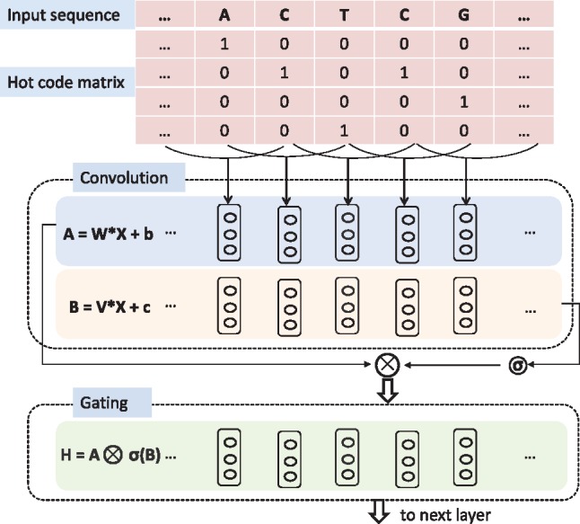
Each nucleotide of the sequence is converted to a four-element vector with one element setting to one and others setting to zero. The output of each hidden layer is a gated convolutional layer where one convolution layer is modulated by another convolution layer through a sigmoid gate

2.5 Gated inception networks

The advantages of the Inception models and gated convolutional networks inspired us to design a new network in order to fuse these advantages. This network architecture enables the predictor to seize local motifs of nucleosome DNA sequences as well as to capture the long-range association between nucleotides. We have tried dozens of versions of network structure. The version finally selected as the network of LeNuP is depicted in Figure 5. Figure 4a–c show the detailed components used in Figure 5. Some details of the LeNup structure partially shown in Figures 4 and 5 are explained and summarized as follows:

Fig. 5.

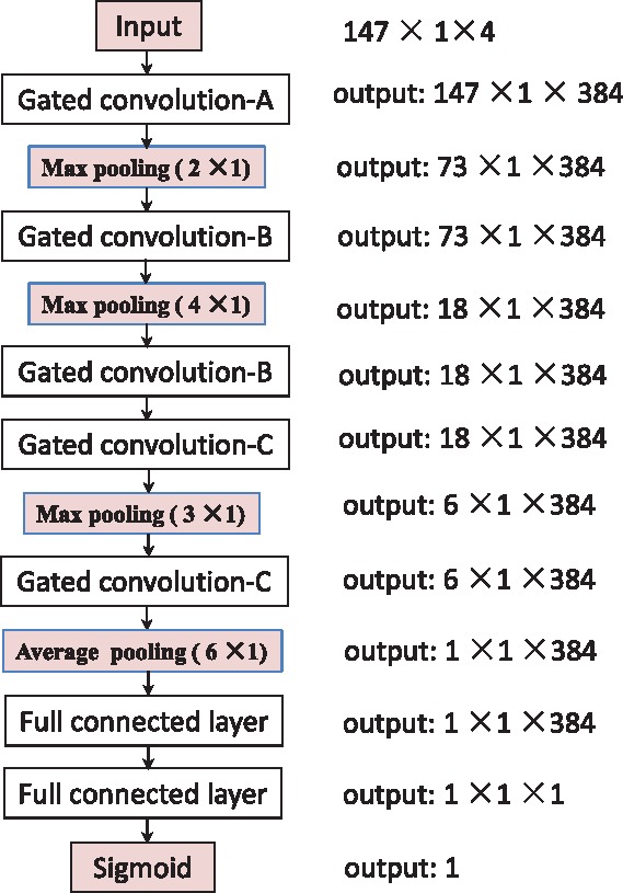
The overall schema of LeNup. For the detailed modules, please refer to Figure 4a–c for the detailed structure of the various components

Fig. 4.

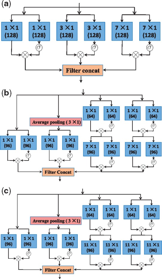
The schema of Gated Inception blocks used in Figure 5: (a) Gated convolution-A block; (b) Gated convolution-B block; (c) Gated convolution-C block

1. Each input tensor is 147 in width, 1 in height and 4 in depth.

2. The convolution operation comes in pairs. As a gate limitation, one of them passes through a sigmoid function to control another operator result.

3. All convolution results in Figure 4a–c are passed through the rectified linear unit (ReLU) for activation, which are not shown in these figures.

4. m × 1, such as 1 × 1, 3 × 1, means that the filter has m in width and 1 in height. The depth of filters is not shown here, which depends on how many filters used in the previous layer. The number 128 or 96 in the parenthesis beneath m × 1 means the convolution with 128 filters or 96 filters. Therefore, the depth of the output of this layer will be 128 or 96.

5. An average pooling layer or a maximum pooling layer with m × 1 means that the pooling stride is m.

6. The block of Filter Concat in all figures means that the operation stacks all features from each branch together. For instance, Figure 4a shows that each gated convolutional subnetwork produces 128 features. We get 128 × 3 = 384 features through the filter concatenation.

7. The output such as 73 × 1 × 384 in Figure 5 means that the dimension of feature maps is 73 in width, 1 in height and 384 in depth.

8. One dropout layer with 30% of dropped outputs was performed after each pooling operation in LeNup.

9. We used a linear layer with sigmoid loss as the classifier.

2.6 Training methodology

We have trained our networks running on a single NVidia Quadro M5000 GPU and implemented our models with stochastic gradient descent with momentum in Torch7 (http://torch.ch). Torch7 is a versatile numeric computing framework and machine learning library that extends Lua. We paid attention to exploring the hyperparameter space of models to identify a compact model with good generalization performance. Our experiments used momentum with a decay of 0.98. We used a learning rate of 0.002, and decayed every epoch using an exponential rate of 0.97.

3 Results and discussion

3.1 Rule of performance evaluating

We used training datasets to train the predictor based upon our gated Inception networks. To survey the generalization performance, the predictor was tested by test datasets which are independent on training datasets. We defined the nucleosome-forming sequences as positive samples and the nucleosome-inhibiting sequences as negative samples. In this work, we adopted the sensitivity (S_n), the specificity (S_p), the accuracy (ACC) and the Matthew’s correlation coefficient (MCC) to score the predictive performance of the corresponding method. They are defined as follows:

$$\begin{array}{l}{S}_n=\frac{T_p}{T_p+F_n}\\ S_p=\frac{T_n}{T_n+F_p}\\ ACC=\frac{T_p+T_n}{T_p+F_n+T_n+F_p}\\ MCC=\frac{T_p\times T_n-F_p\times F_n}{\sqrt{(T_n+F_n)\times (T_n+F_p)\times (T_p+F_n)\times (T_p+F_p)}}\end{array}$$ (3)

where T_p, T_n, F_p and F_n are the numbers of true positives, true negatives, false positives and false negatives, respectively. S_n ∈ [0, 1], S_p ∈ [0, 1], ACC ∈ [0, 1] and MCC ∈ [– 1, 1]. S_n = 0 means that all positives predict to the negatives. When all predictions are incorrect, therefore, T_p = 0 and T_n = 0, we have S_n = 0, S_p = 0, ACC = 0 and MCC = – 1. When all predictions are correct, thus F_p = 0, and F_n = 0, we have S_n = 1, S_p = 1, ACC = 1 and MCC = 1. When all positives are correctly predicted and all negative predictions are wrong, we have S_n = 1, S_p = 0 and MCC = 0. When all negatives are correctly predicted and all positive predictions are wrong, we have S_p = 1, S_n = 0 and MCC = 0. When $\frac{T_p}{F_n}=\frac{F_p}{T_n}=1$, therefore, S_n = S_p = ACC = MCC = 0.5, the predictor is not better than a random choice. We calculated all evaluation indices according to the test result.

We also used ROC curve (receiver operating characteristic curve) to illustrate the performance of the binary classifier LeNup. The curve is created by plotting the sensitivity (S_n) against the false-positive rate (1–S_p) at various threshold settings. The area under the curve (AUC) represents the probability that a classifier will rank a randomly chosen positive instance higher than a randomly chosen negative one. Usually 0.5 < AUC < 1. The closer the AUC value is to 1, the better the classifier performance.

3.2 LeNup performance

We utilized the 20-fold cross validation to evaluate our predictor. The benchmark datasets of each organism (Guo et al., 2014), that is, H. sapiens, C. elegans and D. melanogaster, were randomly divided into 20 data subsets of approximately equal size. We trained the network 20 times. For every training, one of the 20 sub-datasets was used as the test dataset and the others were combined to form the training dataset. All evaluation indices of our predictor, that is, S_n, S_p, ACC, MCC and AUC, are calculated according to test results in our work. The average values of four metrics S_n, S_p, ACC and MCC defined in Equation (3) over 20 test datasets are listed in Table 1 for the LeNup predictor. Figure 6 shows the ROC curves. The area under the curves, or AUC, is 0.9412, 0.9653 and 0.9401 for H. sapiens, C. elegans and D. melanogaster, respectively.

Table 1.

LeNup performance measured by four metrics via 20-fold cross validation

Species	Sn	Sp	ACC	MCC	AUC
H. sapiens	0.9212	0.8562	0.8889	0.7906	0.9412
C. elegans	0.9339	0.9041	0.9188	0.8444	0.9653
D. melanogaster	0.8974	0.8713	0.8847	0.7828	0.9401

Note: The datasets were downloaded from the Supplementary Material of Guo et al., 2014.

Fig. 6.

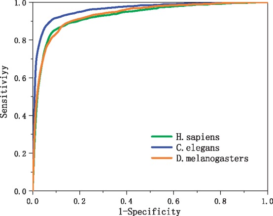
ROC curves obtained from 20-fold cross-validation tests using the genome dataset of H. sapiens, C. elegans and D. melanogaster

3.3 Comparison of LeNup predictions to other algorithms

We compared the performance of our predictor to two recently published predictors with the same benchmark datasets. 3LS was developed by the linear regression model. iNuc-PseKNC is based on SVM. Table 2 shows that the performance of LeNup is much better than 3LS, iNuc-STNC (Tahir et al., 2016), and iNuc-PseKNC for C. elegans and D. melanogaster. For D. melanogaster, compared with 3LS, and iNuc-PseKNC, Matthew’s correlation coefficient (MCC) increased by 17.1% and 30.4%, respectively, the accuracy (ACC) increased by 6.06%, and 10.63%, respectively. For C. elegans, compared with 3LS and iNuc-PseKNC, MCC increased by 11.4%, and 14.1%, respectively, ACC increased by 4.57%, and 5.73%, respectively. For H. sapiens, compared with iNuc-PseKNC, MCC increased by 8.3% and ACC increased by 3.03%. For H. sapiens, LeNup performs slightly worse than 3LS, MCC and ACC decreased by 1.24%. LeNup exhibited perfect performance for the nucleosome positioning prediction. Using the benchmark dataset of yeast genome (Chen et al., 2016), we achieved S_n = S_p = ACC = MCC = 1.0 using 20-fold cross validation. For the same benchmark dataset, the predictor based on DNA deformation energy (Chen et al., 2016) had S_n = 0.982, S_p = 0.980, ACC = 0.981, MCC = 0.963.

Table 2.

Comparison of LeNup predictions to other predictors

Species	Predictor	Sn	Sp	ACC	MCC	AUC
H. sapiens	LeNup	0.9212	0.8562	0.8889	0.7906	0.9412
	3LS	0.9169	0.8835	0.9001	0.8006	0.9588
	iNuc-PseKNC	0.8786	0.8470	0.8627	0.73	0.925
	iNuc-STNC	0.8931	0.8591	0.8760	0.75
C. elegans	LeNup	0.9339	0.9041	0.9188	0.8444	0.9663
	3LS	0.8654	0.8921	0.8786	0.7576	0.9505
	iNuc-PseKNC	0.9030	0.8355	0.8690	0.74	0.935
	iNuc-STNC	0.9162	0.8666	0.8862	0.77
D. melanogaster	LeNup	0.8974	0.8713	0.8847	0.7828	0.9401
	3LS	0.8407	0.8274	0.8341	0.6682	0.9147
	iNuc-PseKNC	0.7831	0.8165	0.7997	0.60	0.874
	iNuc-STNC	0.7976	0.8361	0.8167	0.63

3.4 Impact of cross-validation

3LS and iNuc-PseKNC used a Jackknife test for the cross-validation. During the process of the Jackknife test, each sequence is singled out in turn as a test sample, the remaining sequences are used as training set to calculate test sample’s membership and predict the class. The convolutional neural network as shown in Figures 4 and 5 includes 2 026 880 filter parameters. Training them is very time-consuming, therefore, it is unrealistic to adopt the Jackknife test for the cross-validation. The Jackknife test used by 3LS and iNuc-PseKNC is the extreme situation of k-fold cross validation where k is equal to the total number of sequences in the dataset. We chose k = 5, 10, 20 and 40 to survey the effect of k in k-fold cross validation. Table 3 shows the performance of LeNup with the different k for H. sapiens. As we thought, the performance if gradually improved with the increase of k, because of the training dataset including more training samples with a bigger k. The Matthew’s correlation coefficient of LeNup is 2.32% higher than 3LS predictor, and 12.2% higher than iNuc-PseKNC predictor for the 40-fold cross validation. It is highly possible that the performance of LeNuP can be further improved if we expand the training dataset.

Table 3.

LeNup performance measured by four metrics via 5, 10, 20, 40-fold cross validation

k	Sn	Sp	ACC	MCC
5	0.9024	0.8511	0.8768	0.7695
10	0.9092	0.8486	0.8786	0.7726
20	0.9212	0.8562	0.8889	0.7906
40	0.9335	0.8756	0.9045	0.8192

3.5 SVM classification and Jackknife test

Support vector machine is a more powerful classifier, and it has excellent generalization ability. However, if we used SVM as the classifier instead of the sigmoid function during the training of LeNup, the training time of the model could be several years. We can use LeNup to output the final features of DNA fragment, and then employ SVM to classify the features. Therefore, We used LeNup as a tool to automatically extract features from DNA fragments with 147 bp in length. All 384 features (Supplementary Material) for every DNA fragment in the benchmark datasets of nucleosome forming and inhibiting sequences (Awazu, 2017; Guo et al., 2014) were output from the full connected layer as shown in Figure 5 once the prediction accuracy converged or the overfitting occurred in the test dataset. The overfitting means that the classification accuracy in the training dataset is much better than the test accuracy in the test dataset when we performed LeNup through k-fold cross validation, k = 20 here. After that, the LIBSVM 3.22 package (Fan et al., 2005) was employed as an implementation of SVM with the Gaussian kernel function. The Jackknife test was adopted to examine the performance, where each feature vector in the dataset was in turn singled out as an independent test sample and performed the model training on the remaining data. S_n, S_p, ACC and MCC were evaluated for human, worm and fly genome benchmark datasets (Table 4). The prediction evaluation index shown in Table 4 indicates that the performance of LeNup combining with SVM is far beyond the performance of the recently proposed predictors which are shown in Table 2.

Table 4.

SVM classification and Jackknife test

Species	Sn	Sp	ACC	MCC
H. sapiens	0.9825	0.9827	0.9826	0.9653
C. elegans	0.9961	0.9938	0.9949	0.9899
D. melanogaster	0.9949	0.9943	0.9942	0.9884

3.6 Robustness of LeNup prediction

A benchmark dataset is randomly partitioned into k subsets of approximately equal size to generate the training dataset and the test dataset. The randomness of the data partition leads to the perturbation of training datasets and test datasets between different batches of data partition. To survey the effect of dataset random partition. We produced 5 batches datasets which included 20 subsets from the benchmark dataset of H. sapiens. We trained and tested LeNup using each dataset with 20-fold cross validation. Supplementary Table S1 shows the sample variance of S_n, S_p, ACC and MCC. These variances are five to six orders of magnitude smaller than the average value shown from Tables 1–3. Therefore, we believe that the effect of the randomness of the data partition can be ignored.

3.7 LeNup validates the preference of nucleotide and dinucleotide in nucleosome regions

We scanned the human genome with the previously trained LeNup. The sequence of human chromosome 20 from hg18 version was scanned with stride 1 to 62 435 819 DNA fragments, and the length for each of them is 147 bp. LeNup output the probability of each DNA fragment. We assume that a DNA fragment is a nucleosome preferred position if the probability is greater than 0.85, or it is a nucleosome undesirable position if the probability is less than 0.15. We obtained 25 250 319 nucleosome preferred fragments and 26 950 803 nucleosome undesirable fragments. We calculated the percentage of every nucleotide and dinucleotide in two sorted fragments (Fig. 7). The content of A, T, G, C in the nucleosome preferred fragments is 25.32%, 25.22%, 24.87% and 24.58%, respectively, and the content of A, T, G, C in the nucleosome undesirable fragments is 30.18%, 30.65%, 19.61% and 19.65%, respectively, (Fig. 7a). Figure 7 indicates that nucleosomes preferentially associate with DNA segments exhibiting high CC and GG content, with some degree of exclusion from corresponding A, T, AA and TT rich regions. These predictions are consistent with other publications (Bernstein et al., 2004; Valouev et al., 2011).

Fig. 7.

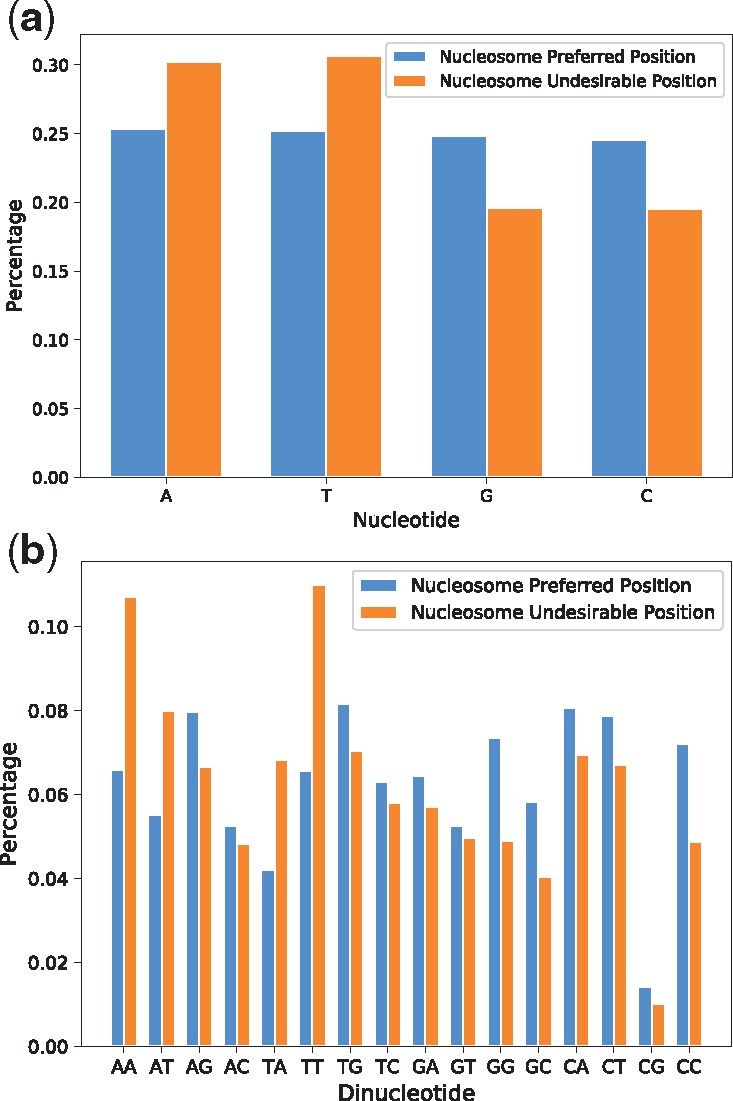
The preference of nucleotide and dinucleotide in nucleosome preferred regions and nucleosome undesirable regions

3.8 LeNup predicts nucleosomes near transcription start sites

We downloaded 1215 transcription start sites (TSSs) for human chr20 genome from UCSC Genome Browser (http://genome.ucsc.edu/cgi-bin/hgTables). The nucleosome distribution profiles between –1000 bp to 1000 bp around each TSS were predicted by the previously trained LeNup. Supplementary Figure S1 shows the average distribution profile of nucleosome near the TSSs. LeNup predicts that nucleosomes are depleted in the region near the TSSs (Rach et al., 2011). The region may be nucleosome free for expressed genes (Lee et al., 2004; Valouev et al., 2011). Supplementary Figure S1 shows well-positioned +1 nucleosome in the promoter regions. The prediction indicates that the –1 nucleosome probability is intensively lower than +1 nucleosome probability, which has been confirmed existing simultaneously in the active and inactive promoters (Schones et al., 2008), suggesting a potential role in maintaining the nucleosome free region.

3.9 LeNup was further tested by MNase-seg results

We compared our model predictions with MNase-seg results (Supplementary Table S2). Nucleosome score profile for human chr20 in activated CD4 cell was downloaded from https://dir.nhlbi.nih.gov/papers/lmi/epigenomes/hgtcellnucleosomes.aspx. There is a score every 10 base span from nucleotide base position 8006 to 62435275. In general, the higher the score value, the bigger the possibility which the position is occupied by a nucleosome. We obtained nucleosome-preferring sequences by scanning the score profile with a score threshold, mapping the local peak positions of the profile to the genome sequence to get the centers of the nucleosome sequences and extending 73 bases at each side of the centers. We took the score threshold as 2, 5, 10, 15, 20, 25, and 30, and got 143 189, 119 857, 67 569, 28 706, 11 209, 3807 and 1375 nucleosome-preferring sequences, respectively. We input these sequences to the previously trained LeNup with the training dataset mentioned in Table 1. Corresponding to these input nucleosome sequences, our model predicted that 109 930, 99 107, 61 730, 27 467, 10 794, 3744, 1362 sequences are nucleosome-preferring sequences among them. The ratio of the predictions to MNase-seg experiments are 0.768, 0.827, 0.914, 0.957, 0.963, 0.984 and 0.991, respectively.

We scanned the zero score regions in the score profile and mapped the regions to the genome to obtain nucleosome-inhibiting sequences. We got 80 563 sequences with a length of 147 bp in this way. We input these sequences to the same model used above. It output 66 421 nucleosome-inhibiting sequences among them, and the ratio of the model predictions to MNase-seq results is 0.825.

4 Conclusion

Our results yield a solid evidence that Inception-like convolutional neural network with a gating mechanism is a viable method for improving the prediction of nucleosome positioning. The main advantage of this method is automatically learning the feature representation compared to other classification algorithms such as support vector machine depending on the external feature extraction. Furthermore, it can be noted that our method has the competitive advantage over other recently published methods. This success suggests promising opportunities for understanding the genetic determinants.

References

- Awazu A. (2017) Prediction of nucleosome positioning by the incorporation of frequencies and distributions of three different nucleotide segment lengths into a general pseudo k-tuple nucleotide composition. Bioinformatics, 33, 42–48. [DOI] [PMC free article] [PubMed] [Google Scholar]
- Barski A. et al. (2007) High-resolution profiling of histone methylations in the human genome. Cell, 129, 823–837. [DOI] [PubMed] [Google Scholar]
- Bell O. et al. (2011) Determinants and dynamics of genome accessibility. Nat. Rev. Genet., 12, 554–564. [DOI] [PubMed] [Google Scholar]
- Bengio Y. et al. (2013) Representation learning: a review and new perspectives. Pattern Anal. Mach. Intell. IEEE Trans., 35, 1798–1828. [DOI] [PubMed] [Google Scholar]
- Bernstein B.E. et al. (2004) Global nucleosome occupancy in yeast. Genome Biol., 5, R62. [DOI] [PMC free article] [PubMed] [Google Scholar]
- Brogaard K. et al. (2012) A map of nucleosome positions in yeast at base-pair resolution. Nature, 486, 496–501. [DOI] [PMC free article] [PubMed] [Google Scholar]
- Chen W. et al. (2012) iNuc-PhysChem: a sequence-based predictor for identifying nucleosomes via physicochemical properties. PLoS One, 7, e4784. [DOI] [PMC free article] [PubMed] [Google Scholar]
- Chen W. et al. (2016) Using deformation energy to analyze nucleosome positioning in genomes. Genomics, 107, 69–75. [DOI] [PubMed] [Google Scholar]
- Chou K.C. (2001) Prediction of protein cellular attributes using pseudo-amino acid composition. PROTEINS Struct. Funct. Genet., 43, 246–255. [DOI] [PubMed] [Google Scholar]
- Chou K.C. (2005) Using amphiphilic pseudo amino acid composition to predict enzyme subfamily classes. Bioinformatics, 21, 10–19. [DOI] [PubMed] [Google Scholar]
- Collobert R. et al. (2011a) Natural language processing (almost) from scratch. J. Mach. Learn. Res., 12, 2493–2537. [Google Scholar]
- Dauphin Y.N. et al. (2016) A Language modeling with gated convolutional networks. arXiv: 1612.08083v1.
- Eaton M.L. et al. (2010) Conserved nucleosome positioning defines replication origins. Genes Dev., 24, 748–753. [DOI] [PMC free article] [PubMed] [Google Scholar]
- Esteva A. et al. (2017) Dermatologist classification of skin cancer with deep neural networks. Nature, 542, 115–118. [DOI] [PMC free article] [PubMed] [Google Scholar]
- Fan R.E. et al. (2005) Working set selection using second order information for training support vector machines. J. Mach. Learn. Res., 6, 1889–1918. [Google Scholar]
- Field Y. et al. (2008) Distinct modes of regulation by chromatin encoded through nucleosome positioning signals. PLoS Comput. Biol., 4, e1000216. [DOI] [PMC free article] [PubMed] [Google Scholar]
- Guertin M.J., Lis J.T. (2013) Mechanisms by which transcription factors gain access to target sequence elements in chromatin. Curr. Opin. Genet. Dev., 23, 116–123. [DOI] [PMC free article] [PubMed] [Google Scholar]
- Guo S. et al. (2014) iNuc-PseKNC: a sequence-based predictor for predicting nucleosome positioning in genomes with pseudo k-tuple nucleotide composition. Bioinformatics, 30, 1522–1529. [DOI] [PubMed] [Google Scholar]
- Gupta S. et al. (2008) Predicting human nucleosome occupancy from primary sequence. PLoS Comput. Biol., 4, e1000134. [DOI] [PMC free article] [PubMed] [Google Scholar]
- Gonzalez S. (2016) Nucleosomal signatures impose nucleosome positioning in coding and noncoding sequences in the genome. Genome Res., 26, 1532–1543. [DOI] [PMC free article] [PubMed] [Google Scholar]
- Hinton G., Salakhutdinov R. (2006) Reducing the dimensionality of data with neural networks. Science, 313, 504–507. [DOI] [PubMed] [Google Scholar]
- Hinton G. et al. (2012) Deep neural networks for acoustic modeling in speech recognition. IEEE Signal Process. Mag., 29, 82–97. [Google Scholar]
- Ioshikhes I. et al. (1996) Nucleosome DNA sequence pattern revealed by multiple alignment of experimentally mapped sequences. J. Mol. Biol., 262, 129–139. [DOI] [PubMed] [Google Scholar]
- Ioshikhes I. et al. (2011) Variety of genomic DNA patterns for nucleosome positioning. Genome Res., 21, 1863–1871. [DOI] [PMC free article] [PubMed] [Google Scholar]
- Jiang C., Pugh B.F. (2009) Nucleosome positioning and gene regulation: advances through genomics. Nat. Rev. Genet., 10, 161–172. [DOI] [PMC free article] [PubMed] [Google Scholar]
- Kaplan N. et al. (2009) The DNA-encoded nucleosome organization of a eukaryotic genome. Nature, 458, 362–366. [DOI] [PMC free article] [PubMed] [Google Scholar]
- Kelley D.R. et al. (2016) Basset: learning the regulatory code of the accessible genome with deep convolutional neural networks. Genome Res., 26, 990–999. [DOI] [PMC free article] [PubMed] [Google Scholar]
- Kornberg R.D., Lorch Y. (1999) Twenty-five years of the nucleosome, fundamental particle of the eukaryote chromosome. Cell, 98, 285–294. [DOI] [PubMed] [Google Scholar]
- Krizhevsky A. et al. (2012) ImageNet classification with deep convolutional neural networks. In Proc. Adv. Neural Information Process. Syst., 25, 1090–1098. [Google Scholar]
- LeCun Y. et al. (2015) Deep learning. Nature, 521, 436–444. [DOI] [PubMed] [Google Scholar]
- Lee C.K. et al. (2004) Evidence for nucleosome depletion at active regulatory regions genome-wide. Nat. Genetics, 36, 900–905. [DOI] [PubMed] [Google Scholar]
- Lee W. et al. (2007) A high- resolution atlas of nucleosome occupancy in yeast. Nat. Genet., 39, 1235–1244. [DOI] [PubMed] [Google Scholar]
- Leung M.K. et al. (2014) Deep learning of the tissue-regulated splicing code. Bioinformatics, 30, i121–i129. [DOI] [PMC free article] [PubMed] [Google Scholar]
- Liu B. et al. (2016) iDHS-EL: identifying DNase I hypersensitive sites by fusing three different modes of pseudo nucleotide composition into an ensemble. Bioinformatics, 32, 2411–2418. [DOI] [PubMed] [Google Scholar]
- Liu M. et al. (2015) Determinants of nucleosome positioning and their influence on plant gene expression. Genome Res., 25, 1182–1195. [DOI] [PMC free article] [PubMed] [Google Scholar]
- Liu S. et al. (2017) RPA binds histone H3-H4 and functions in DNA replication-coupled nucleosome assembly. Science, 355, 415–420. [DOI] [PubMed] [Google Scholar]
- Luger K. et al. (1997) Crystal structure of the nucleosome core particle at 2.8 Å resolution. Nature, 389, 251–260. [DOI] [PubMed] [Google Scholar]
- Mavrich T.N. et al. (2008) Nucleosome organization in the Drosophila genome. Nature, 453, 358–362. [DOI] [PMC free article] [PubMed] [Google Scholar]
- Miele V. et al. (2008) DNA physical properties determine nucleosome occupancy from yeast to fly. Nucleic Acids Res., 11, 3746–3756. [DOI] [PMC free article] [PubMed] [Google Scholar]
- Minary P., Levitt M. (2014) Training-free atomistic prediction of nucleosome occupancy. Proc. Natl. Acad. Sci. USA, 111, 6293–6298. [DOI] [PMC free article] [PubMed] [Google Scholar]
- Morozov A.V. et al. (2009) Using DNA mechanics to predict in vitro nucleosome positions and formation energies. Nucleic Acids Res., 37, 4707–4722. [DOI] [PMC free article] [PubMed] [Google Scholar]
- Pulivarthy S.R. et al. (2016) Regulated large-scale nucleosome density patterns and precise nucleosome positioning correlate with V(D)J recombination. Proc. Natl. Acad. Sci. USA, 113, E6427–E6436. [DOI] [PMC free article] [PubMed] [Google Scholar]
- Rach E.A. et al. (2011) Transcription initiation patterns indicate divergent strategies for gene regulation at the chromatin level. PLoS Genetics, 7, e1001274. [DOI] [PMC free article] [PubMed] [Google Scholar]
- Richmond T.J., Davey C.A. (2003) The structure of DNA in the nucleosome core. Nature, 423, 145–150. [DOI] [PubMed] [Google Scholar]
- Satchwell S.C. et al. (1986) Sequence periodicities in chicken nucleosome core DNA. J. Mol. Biol., 191, 659–675. [DOI] [PubMed] [Google Scholar]
- Schones D.E. et al. (2008) Dynamic regulation of nucleosome positioning in the human genome. Cell, 132, 887–898. [DOI] [PMC free article] [PubMed] [Google Scholar]
- Segal E. et al. (2006) A genomic code for nucleosome positioning. Nature, 442, 772–778. [DOI] [PMC free article] [PubMed] [Google Scholar]
- Segal E., Widom J. (2009) What controls nucleosome positions? Trends Genet., 25, 335–243. [DOI] [PMC free article] [PubMed] [Google Scholar]
- Silver D. et al. (2016) Mastering the game of Go with deep neural networks and tree search. Nature, 529, 484–489. [DOI] [PubMed] [Google Scholar]
- Smagulova F. et al. (2011) Genome-wide analysis reveals novel molecular features of mouse recombination hotspots. Nature, 472, 375–378. [DOI] [PMC free article] [PubMed] [Google Scholar]
- Struhl K., Segal E. (2013) Determinants of nucleosome positioning. Nat. Struct. Mol. Biol., 20, 267–273. [DOI] [PMC free article] [PubMed] [Google Scholar]
- Szegedy C. et al. (2015) Going deeper with convolutions. In: Proceedings of the IEEE Conference on Computer Vision and Pattern Recognition, IEEE, Boston, MA, USA, pp. 1–9. [Google Scholar]
- Szegedy C. et al. (2016) Inception-v4, Inception-ResNet and the Impact of Residual Connections on Learning. arXiv: 1602.06271v1.
- Tahir M., Hayat M. (2016) iNuc-STNC: a sequence-based predictor for identification of nucleosome positioning in genomes by extending the concept of SAAC and Chous PseAAC. Mol. Biosyst., 12, 2587. [DOI] [PubMed] [Google Scholar]
- Tilgner H. et al. (2009) Nucleosome positioning as a determinant of exon recognition. Nat. Struct. Mol. Biol., 16, 996–1001. [DOI] [PubMed] [Google Scholar]
- Valouev A. et al. (2008) A high-resolution, nucleosome position map of C. elegans reveals lack of universal sequence-dictated positioning. Genome Res., 18, 1051–1063. [DOI] [PMC free article] [PubMed] [Google Scholar]
- Valouev A. et al. (2011) Determinants of nucleosome organization in primary human cells. Nature, 474, 516–520. [DOI] [PMC free article] [PubMed] [Google Scholar]
- van der Heijden T. et al. (2012) Sequence-based prediction of single nucleosome positioning and genome-wide nucleosome occupancy. Proc. Natl. Acad. Sci. USA, 109, E2514–E2522. [DOI] [PMC free article] [PubMed] [Google Scholar]
- Vasseur P. et al. (2016) Dynamics of nucleosome positioning maturation following genomic replication. Cell Rep., 16, 2651–2665. [DOI] [PMC free article] [PubMed] [Google Scholar]
- Wang J.Y. et al. (2012) Calculation of nucleosomal DNA deformation energy: its implication for nucleosome positioning. Chromosome Res., 20, 889–902. [DOI] [PubMed] [Google Scholar]
- Weiner A. et al. (2009) High-resolution nucleosome mapping reveals transcription-dependent promoter packaging. Genome Res., 2010, 90–100. [DOI] [PMC free article] [PubMed] [Google Scholar]
- Widlund H.R. et al. (1999) Nucleosome structural features and intrinsic properties of the TATAAACGCC repeat sequence. J. Biol. Chem., 274, 31847–31852. [DOI] [PubMed] [Google Scholar]
- Whitehouse L. et al. (2007) Chromatin remodelling at promoters suppresses antisense transcription. Nature, 450, 1031–1035. [DOI] [PubMed] [Google Scholar]
- Xi L.Q. et al. (2010) Predicting nucleosome positioning using a duration Hidden Markov Model. BMC Bioinformatics, 11, 1–9. [DOI] [PMC free article] [PubMed] [Google Scholar]
- Xiong H.Y. et al. (2015) The human splicing code reveals new insights into the genetic determinants of disease. Science, 347, 1254806. [DOI] [PMC free article] [PubMed] [Google Scholar]
- Yuan G.C. et al. (2005) Genome-scale identification of nucleosome positions in S-cerevisiae. Science, 309, 626–630. [DOI] [PubMed] [Google Scholar]
- Yuan G.C., Liu J.S. (2008) Genomic sequence is highly predictive of local nucleosome depletion. PLoS Computat. Biol., 4, e13. [DOI] [PMC free article] [PubMed] [Google Scholar]
- Zhang Y. et al. (2009) Intrinsic histone-DNA interactions are not the major determinant of nucleosome positions in vivo. Nat. Struct. Mol. Biol., 16, 847–852. [DOI] [PMC free article] [PubMed] [Google Scholar]
- Zhong J. et al. (2016) Mapping nucleosome positions using DNase-seq. Genome Res., 26, 351–364. [DOI] [PMC free article] [PubMed] [Google Scholar]
Associated Data
This section collects any data citations, data availability statements, or supplementary materials included in this article.