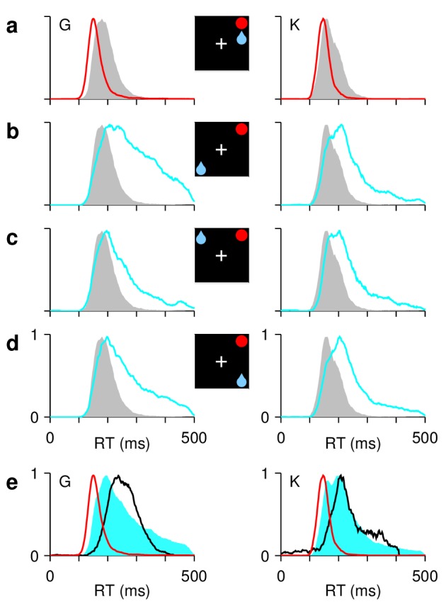
Figure 2. Asymmetric reward expectation leads to strong spatial bias.

(a–d) RT distributions for correct saccades, for monkeys G (left column) and K (right column). Insets indicate rewarded location (blue drop) and target (red circle). When the two are congruent ([a], red traces), RTs are shorter and less variable than when they are incongruent, that is, either opposite ([b], cyan) or adjacent ([c], [d], cyan). In unbiased trials (ADR task; gray), results are intermediate. (e) RT distributions in correct congruent (red, same data as in [a]), correct incongruent (cyan, data in [b-d] combined), and incorrect incongruent (black) trials. Histograms are normalized to a maximum of 1. The RTs during errors are neither the fastest nor the slowest.

Figure 2—figure supplement 1. Variations in spatial bias over time.

Analyses of the sequential responses made by the two animals confirmed that they were strongly aware of which location was the rewarded one. (a, b) Time course of bias adaptation after a change in rewarded location. Mean RT ($\pm$ 1 SE) for saccades to a fixed location as a function of the number of trials before or after a change in reward status (i.e., block transition). Transitions from unrewarded to rewarded (a, red) are faster than from rewarded to unrewarded (b, cyan). Horizontal lines indicate asymptotic RT values. Black lines are exponential fits with time constants as indicated ($\tau$; units are trials). (c, d) Trial history effects. Mean RTs ($\pm$ 1 SE) to rewarded ([c], red) and unrewarded ([d], cyan) targets are shown conditioned on various preceding sequences of rewarded (R) and unrewarded (U) trials. Note systematic changes in RT, which are somewhat idiosyncratic to each animal, as each condition is repeated. For calculating these trial-history effects, the first 15 trials after each block transition were excluded. All data are from correct responses.

Figure 2—figure supplement 2. Impact of reward-location bias on saccade metrics.

All plots compare measurements in congruent (red labels and markers) versus incongruent conditions (blue labels and markers). (a) Endpoints of saccades to a stimulus located at (10${}^{\circ }$, 0${}^{\circ }$) collected during a single session from monkey G. The origin corresponds to the average saccade endpoint. For each data point, the displacement is the distance to the origin. Yellow circles indicate 1 and 2 SDs in displacement from the congruent data. (b) Mean normalized displacement in each experimental session ($n=135$). Displacement values for each session were z-scored, and then congruent and incongruent trials were averaged separately. Colors indicate monkeys (G, gray; K, white). The session shown in (a) is marked by the green cross. (c) Mean normalized displacement for each monkey, averaged across sessions. Error bars indicate $\pm$ 1 SE. (d) Average time course of eye velocity for saccades to stimuli at (8${}^{\circ }$, 4${}^{\circ }$) collected during a single session from monkey K. Inset zooms in on the change in peak velocity of $\sim {40}^{\circ }$/s between congruent (red, $n=104$ trials) and incongruent (blue, $n=427$ trials) trials. Shades indicate $\pm$ 1 SE across trials. (e) Mean peak velocity in each experimental session. Colors indicate monkeys (G, gray; K, white). The session shown in (d) is marked by the green cross. (f) As in (e) but for saccade amplitude. (g) Average velocity (top) and amplitude (bottom) values averaged across sessions and monkeys. Error bars indicate $\pm$ 1 SE. All significance values are for differences in means across experimental conditions, from permutation tests for paired data. The results indicate that saccades to high-reward locations are spatially more precise (a–c) and have higher peak velocities (d, e, g) than those to low-reward locations, whereas saccade amplitude changes little in comparison (f, g). Results are consistent with earlier reports (Lauwereyns et al., 2002; Takikawa et al., 2002; Watanabe and Hikosaka, 2005).