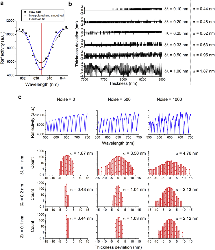
Figure 5.

Testing the precision of the thickness fitting algorithm with reflectance data produced by transfer matrix calculations. Different interpolation conditions and different amounts of Gaussian noise added to the data are compared. (a) A comparison of typical raw data (with Noise = 500, see below), interpolated and smoothed data, and a Gaussian peak fit to the raw data is shown. Red symbols mark the minima in each corresponding data set. The red line indicates the minimum of the Gaussian fit. (b) The difference between nominal and fitted thickness for different increments of wavelength interpolation δλ is shown. σ is the standard deviation of the difference between nominal cavity thickness and fitted thickness. (c) The difference in thickness for different δλ and different amounts of Gaussian noise added to the transfer matrix calculations (standard deviation of noise 0, 500, and 1000) is given. The blue profiles (top) illustrate how the added noise affects the reflectance spectra (cavity thickness, 8000 nm). Note that for noise = 1000 and δλ = 1 nm, the total fraction of pixels in the image that can be fitted at all is only 20%. To see this figure in color, go online.