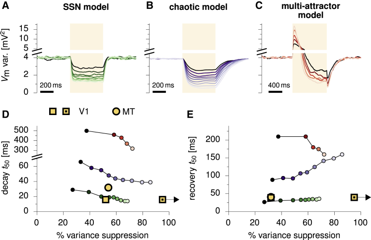
Figure 7.

Temporal Dynamics of Variability Modulation in the SSN versus Other Models

(A) Time course of variability reduction and recovery in the ring SSN in response to a step input (shaded area, 500 ms duration) of increasing amplitude (dark to light). Variability is quantified by the population-averaged across-trial $V_{\text{m}}$ variance.

(B) Same as (A), for chaotic network dynamics (Rajan et al., 2010).

(C) Same as (A), for a continuous, multi-attractor network (Ponce-Alvarez et al., 2013). The stimulus is twice as long as in (A) and (B), so that variability suppression can be observed following the characteristic transient increase.

(D) Timescale of variability suppression (time to reach half of the total suppression) as a function of the percentage of variance suppression in the three models, extracted from their corresponding variability trajectories (colors as in A–C).

(E) Same as (D), for recovery timescales (time to recover half of the total suppression). In both (D) and (E), open yellow squares indicate V1 data from anesthetized cat (estimated from Figure S4 in Churchland et al., 2010); yellow circles show data from anesthetized monkey MT (Figure S4 in Churchland et al., 2010); dotted yellow circles show our analysis of the awake monkey V1 data of Ecker et al., 2010. Variability refers to the above-Poisson part of spike count variability (i.e., population-averaged Fano factor minus one), and time constants discard latencies in data. In the data of Ecker et al., 2010, the Fano factor dropped below one, effectively resulting in $>100\text{\%}$ variance suppression with our definition (right-pointing arrows). All results regarding the SSN and the multi-attractor model shown in this figure were obtained by using the same parameters as in previous figures (Figures 4, 5, and 6).