Figure - PMC

Skip to main content

An official website of the United States government

Here's how you know

Here's how you know

Official websites use .gov
A .gov website belongs to an official government organization in the United States.

Secure .gov websites use HTTPS
A lock ( ) or https:// means you've safely connected to the .gov website. Share sensitive information only on official, secure websites.

View full-text article in PMC

. 2018 May 29;8:8219. doi: 10.1038/s41598-018-26543-w

Search in PMC
Search in PubMed
View in NLM Catalog
Add to search

© The Author(s) 2018

Open Access This article is licensed under a Creative Commons Attribution 4.0 International License, which permits use, sharing, adaptation, distribution and reproduction in any medium or format, as long as you give appropriate credit to the original author(s) and the source, provide a link to the Creative Commons license, and indicate if changes were made. The images or other third party material in this article are included in the article’s Creative Commons license, unless indicated otherwise in a credit line to the material. If material is not included in the article’s Creative Commons license and your intended use is not permitted by statutory regulation or exceeds the permitted use, you will need to obtain permission directly from the copyright holder. To view a copy of this license, visit http://creativecommons.org/licenses/by/4.0/.

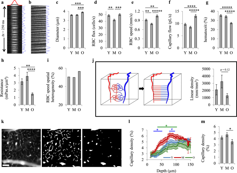
PMC Copyright notice

Capillary blood flow. (a) A representative space-time image from perpendicular scans. The image was averaged in vertical direction and fitted with a Gaussian function (top) to estimate the capillary diameter. The image was also averaged in horizontal direction (right) to find the number of passing RBCs. (b) A representative space-time image from longitudinal scans. RBC velocity was calculated from the angle of dark streaks. The image was rotated by this angle and averaged (right) to find the number of passing RBCs. (c–g) Capillary diameter (c), RBC flux (d) and RBC speed (e) were obtained from space-time images. Capillary volumetric flow (f) and hematocrit (g) were calculated from diameter, flux and speed (Y, n = 242; M, n = 252; O, n = 278 capillaries). (h) Capillary resistance was estimated from diameter and hematocrit. (i) Spatial heterogeneity (defined as the coefficient of variation) of RBC speed. (j) For the mice that both flow in large vessels and capillary flow were measured over the same region (Y, n = 8; M, n = 7; O, n = 8 mice), capillary linear density was estimated (right) by simplifying the capillary network architecture as straight tubes with uniform length and diameter connecting an arteriole to a venule (left). (k) Microvascular angiograms were used to directly obtain the capillary density. Left: an en face slice at the depth of ~80 µm (scale bar: 100 µm). Middle: binarization of the left image. Right: the same as middle image, but processed with a median filter to remove the fine structures (capillaries). (l) Capillary density (volume%) versus depth obtained from angiograms by subtracting the density of large vessels from total vascular density. The blue * (or #) represents statistically significant (or nearly significant) differences between Y and M. The green * represents statistically significant differences between M and O. (m) Average capillary density through the depth of 0–150 µm (Y, n = 18; M, n = 15; O, n = 16 angiograms). Results are presented as mean ± s.e.m. Statistical significance was calculated using ANOVA followed by Tukey HSD post hoc test. *****p < 0.00001, ****p < 0.0001, ***p < 0.001, **p < 0.01, *p < 0.05, ^#p-value approaches significance (p < 0.1). Y: young (8 mice), M: middle-aged (7 mice), O: old (8 mice).