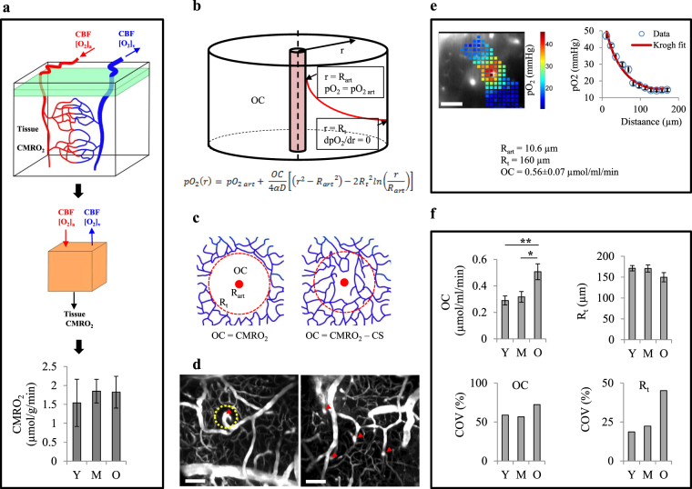
Figure 6.
Estimation of cerebral metabolic rate of oxygen consumption (CMRO2) and net oxygen consumption rate (OC) in tissue. (a) CMRO2 was obtained using the equation CMRO2 = CBF([O2]a-[O2]v) for the mice that both vascular pO2 and blood flow in large vessels were measured over the same region (Y, n = 8; M, n = 7; O, n = 7 mice). (b) The Krogh cylinder model of O2 diffusion from a vessel to surrounding tissue. This model assumes that an infinitely long arteriole with radius Rart supplies an infinitely long tissue cylinder with radius Rt. Continuity equation for O2 is solved assuming a uniform net oxygen consumption rate (OC) in tissue cylinder with specified boundary conditions. (c) If there is a capillary depleted cylinder around arterioles and the major tissue pO2 gradient around arterioles occurs within this region, OC term in Krogh model will be a good estimate of CMRO2 (left). But if the capillary depleted region is much smaller than Rt, OC represents the difference between CMRO2 and capillary O2 supply (CS) (right). (d) Examples of the maximum intensity projection of microvascular angiograms showing diving arterioles (arrow heads) with (left) and without (right) a capillary depleted region; in mice the absence of capillary depleted regions around some arterioles was observed. Even in cases where a capillary depleted region existed, its radius did not exceed 50 µm, while tissue pO2 profiles often saw a significant pO2 drop up to 100 µm from arterioles. (e) 2D-grid point measurements around arterioles (left) yielded pO2 gradients from arterioles which were fitted with the Krogh model to obtain OC (right). (f) OC and Rt were found for individual vessels and were averaged in each age group (top). Spatial heterogeneity of OC and Rt were estimated by the coefficient of variation (bottom) (Y, n = 26 arterioles from 5 mice; M, n = 20 arterioles from 5 mice; O, n = 37 arterioles from 7 mice). Y: young, M: middle-aged, O: old. Scale bars are 100 µm. Bar plots represent mean ± s.e.m. Statistical significance was calculated using ANOVA followed by Tukey HSD post hoc test. **p < 0.01 *p < 0.05.

