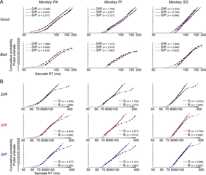
Fig 3. Distribution of SacRTs in different contexts and for different targets.
(A) Distributions of the SacRT for three groups of scenes are superimposed: D/R, S/R, and S/P (see Fig 1C). They are shown separately for the good and bad objects. Data are shown for monkeys PA (left), PI (center), and SO (right) after learning (>350, >200, and >200 trials for each environment, respectively). (B) The same SacRT data are shown separately for the three groups of scenes (D/R, S/R, S/P), but data for good (G) and bad (B) objects are superimposed. The numbers of saccades examined are shown in each graph. The effects of scenes (A) and objects (B) on SacRT were independent and orthogonal in all subjects (two-way ANOVA, monkey PA [scene, F(2,18693) = 68.004, P < 0.001; object, F(1,18693) = 381.645, P < 0.001; scene*object, F(2,18693) = 5.966, P = 0.003], monkey PI [scene, F(2,12428) = 18.313, P < 0.001; object, F(1,12428) = 1,216.167, P < 0.001; scene*object, F(2,12428) = 21.892, P < 0.001], monkey SO [scene, F(2,27266) = 84.198, P < 0.001; object, F(1,27266) = 584.585, P < 0.001; scene*object, F(2, 27266) = 37.405, P < 0.001]). Data used to generate these plots can be found at https://osf.io/2yq8p/?view_only=97c4b290514348bb91cdbb9ec1c85e09. B, bad; D/R, dangerous and rich; G, good; S/P, safe and poor; S/R, safe and rich; SacRT, saccade reaction time.

