Figure - PMC

Skip to main content

An official website of the United States government

Here's how you know

Here's how you know

Official websites use .gov
A .gov website belongs to an official government organization in the United States.

Secure .gov websites use HTTPS
A lock ( ) or https:// means you've safely connected to the .gov website. Share sensitive information only on official, secure websites.

View full-text article in PMC

. 2018 Jun 8;9:2222. doi: 10.1038/s41467-018-03763-2

Search in PMC
Search in PubMed
View in NLM Catalog
Add to search

© The Author(s) 2018

Open Access This article is licensed under a Creative Commons Attribution 4.0 International License, which permits use, sharing, adaptation, distribution and reproduction in any medium or format, as long as you give appropriate credit to the original author(s) and the source, provide a link to the Creative Commons license, and indicate if changes were made. The images or other third party material in this article are included in the article’s Creative Commons license, unless indicated otherwise in a credit line to the material. If material is not included in the article’s Creative Commons license and your intended use is not permitted by statutory regulation or exceeds the permitted use, you will need to obtain permission directly from the copyright holder. To view a copy of this license, visit http://creativecommons.org/licenses/by/4.0/.

PMC Copyright notice

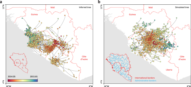
Fig. 2 — Example of a continuous phylogeographic estimate and corresponding simulation. Example of a phylogeographic estimate in continuous space (a) and the corresponding posterior predictive simulation unaware of international borders (b). In both cases, phylogenetic branches are represented by black curves connecting phylogenetic nodes displayed as dots coloured according to their time of occurrence. In a, these nodes are positioned according to the mean latitude and longitude estimates obtained by phylogeographic inference, while in b they are positioned according to simulations based on the estimated parameters of the phylogeographic process. Map background was made in R and based on international borders obtained from the Global Administrative Areas database (GADM, www.gadm.org)