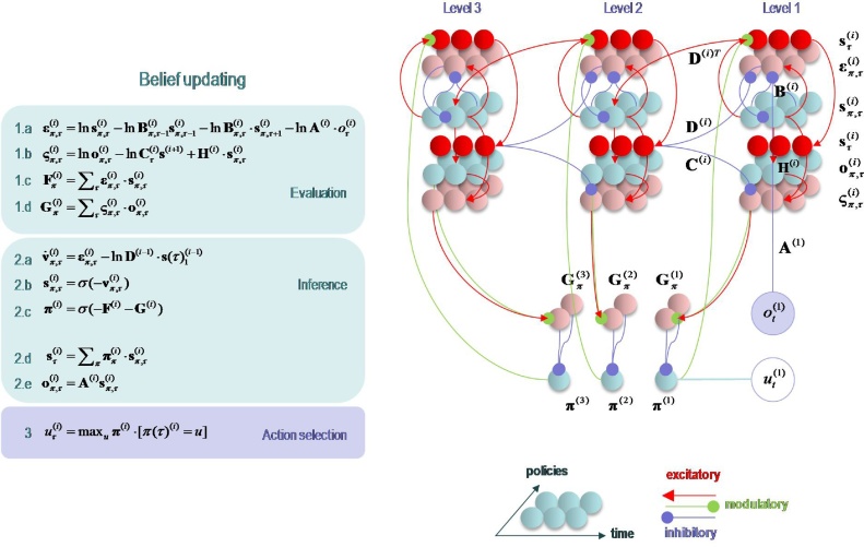
Fig. 2.

Schematic overview of belief propagation: left panel: these equalities are the belief updates mediating inference (i.e. state estimation) and action selection. These expressions follow in a fairly straightforward way from a gradient descent on variational free energy. The equations have been expressed in terms of prediction errors that come in two flavours. The first, state prediction error scores the difference between the (log) expected states under any policy and time (at each hierarchical level) and the corresponding predictions based upon outcomes and the (preceding and subsequent) hidden states (1.a). These represent likelihood and empirical prior terms respectively. The prediction error drives log-expectations (2.a), where the expectation per se is obtained via a softmax operator (2.b). The second, outcome prediction error reports the difference between the (log) expected outcome and that predicted under prior preferences set by the level above (plus an ambiguity term – see Appendix) (1.b). This prediction error is weighted by the expected outcomes to evaluate the expected free energy (1.d). Similarly, the free energy per se is the expected state prediction error, under current beliefs about hidden states (1.c). These policy-specific free energies are combined to give the policy expectations via a softmax function (2.c). Finally, expectations about hidden states are a Bayesian model average over expected policies (2.d) and expectations about policies specify the action that is most likely to realise the expected outcome (3). The (Iverson) brackets in Equation 3 return one if the condition in square brackets is satisfied and zero otherwise. Right panel: this schematic represents the message passing implicit in the equations on the left. The expectations have been associated with neuronal populations (coloured balls) that are arranged to highlight the correspondence with known intrinsic (within cortical area) and extrinsic (between cortical areas) connections. Red connections are excitatory, blue connections are inhibitory and green connections are modulatory (i.e., involve a multiplication or weighting). This schematic illustrates three hierarchical levels (which are arranged horizontally in this figure, as opposed to vertically in Fig. 1), where each level provides top-down empirical priors for the initial state of the level below, while the lower level supplies evidence for the current state at the level above. The intrinsic connections mediate the empirical priors and Bayesian model averaging. Cyan units correspond to expectations about hidden states and (future) outcomes under each policy, while red states indicate their Bayesian model averages. Pink units correspond to (state and outcome) prediction errors that are averaged to evaluate (variational and expected) free energy and subsequent policy expectations (in the lower part of the network). This (neuronal) network interpretation of belief updating means that connection strengths correspond to the parameters of the generative model in Fig. 1. Please see Table 2 for a definition of the variables. The variational free energy has been omitted from this figure because the policies in this paper differ only in the next action. This means the evidence (i.e. variational free energy) from past outcomes is the same for all policies (For interpretation of the references to colour in this figure legend, the reader is referred to the web version of this article).