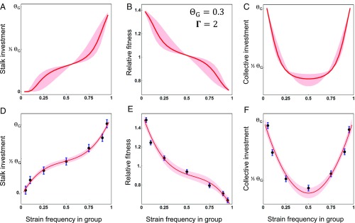
Fig. 4.

Patterns of stalk investment, relative fitness, and collective investment as a function of strain frequencies in chimeric aggregations. A–C illustrate expected patterns under parameter values that resemble the empirical results [using the same equations (Eqs. 11–13) to calculate model expectations as those used for empirical estimation], with the bold line corresponding to the case where ${\mathrm{\Theta }}_{\text{G}}$ = 0.3, Γ = 2, and σ = 0.50, with the shading spanning a range of error in measurement of frequency (relatedness) (σ = 0.25 to σ = 0.75). D–F show empirical results from the set of 34 chimeric pairs (n = 944 total chimeric mixes), with the points representing the means and the bars their SEs, estimated from a mixed model (following the model structure in Materials and Methods, but with frequency as a categorical factor). (D) Individual stalk investment by a focal strain as a function of its frequency in a chimeric aggregation. (E) Relative fitness for a focal strain as a function of its frequency in a chimeric aggregation. (F) Collective investment by chimeras as a function of the frequency of a randomly assigned focal strain to the chimeric aggregation. In D and E the bold curve represents the best-fit estimate from the cubic regression model (here fitted to the estimated means). For F, the curve represents the best-fit estimated from a quadratic regression model (fitted to the estimated means). For all three figures (D–F) the shaded region indicates a one SE interval on either side of the best-fit line. Individual (A and D) and collective (C and F) investment values were rescaled by subtracting $1-{\mathrm{\Theta }}_{\text{G}}$ from the raw measures, under the assumption that ${\mathrm{\Theta }}_{\text{G}}=0.3$ (therefore, the value labeled as ${\mathrm{\Theta }}_{\text{G}}$ corresponds to a value of 0.3 in the figure).