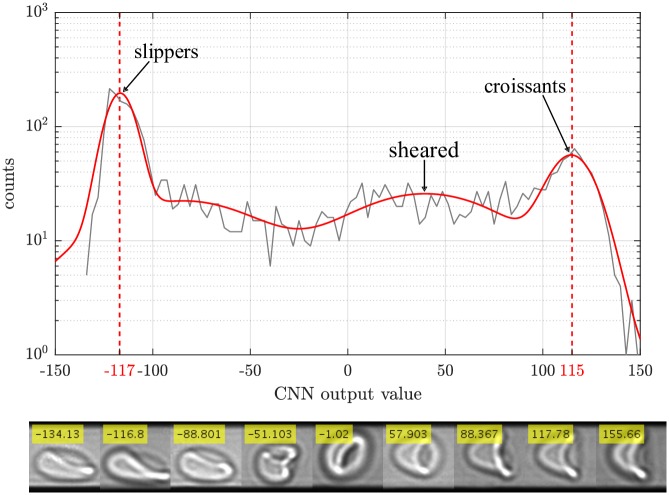
Fig 4. We estimate perfect slippers to be around the peak of the distribution at ≈ −117, whereas croissants occur around ≈ 115.

By fitting the whole spectrum by four Gaussians, we are able to separate the respective contributions of each cell shape class and thus can determine a respective confidence interval. In the lower part, typical cell shapes are depicted for different output value ranges. Starting from the leftmost cell image, we undergo a shape change from slippers (image 1-3) to others (image 4-5) and finally to sheared (image 6-7) and pure croissants (image 8-9).