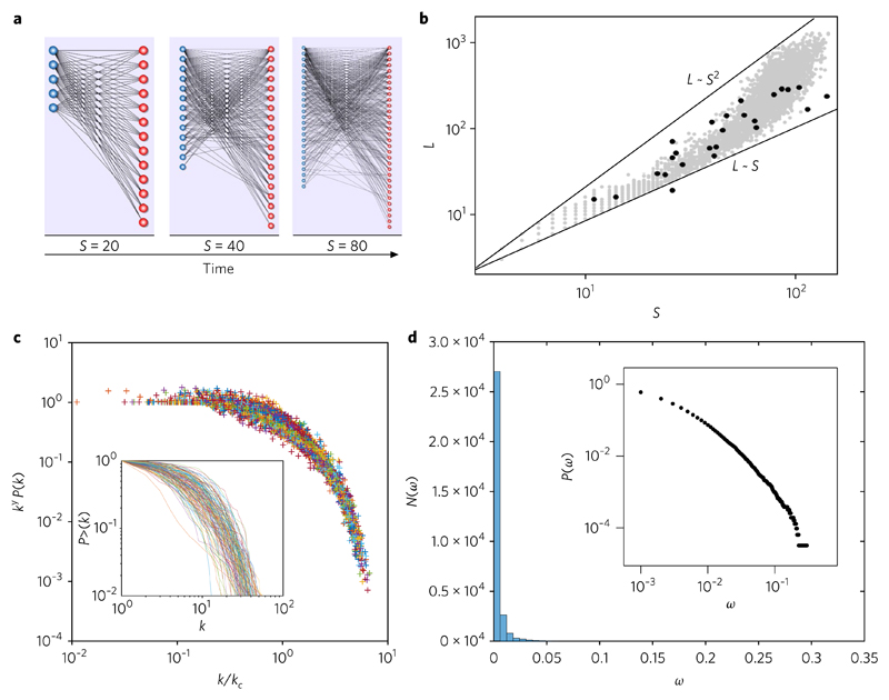
Fig. 2. Connectivity patterns in evolved in silico mutualistic webs.
a, A typical sequence of growing in silico networks with size S = 20, 40, 80 showing a nested pattern that becomes more manifest with time. Here the parameters are β = 10−5, P = 0.1 and θ = 10−6 (pace of evolutionary change, probability of weight change and link removal threshold, respectively). b, Pattern of links–species relationships. The grey dots indicate the (S, L) pairs for each of the m = 4, 000 simulated networks, evolved over T = 500 steps, generated using randomly chosen pairs (p, β). Here, P ∈ (0, 1) and β ∈ (10−4, 10−1). The black dots correspond to our benchmark data and the straight lines provide the limits associated with a purely linear L ~ S and the square L ~ S2 limits, consistent with the mathematical model provided in the Supplementary Information. c, Series of simulated sequences, each of which is collapsed under the truncated power law scaling, P(k) ~ k−γexp(−k/kc). The inset shows the cumulative (undirected) degree distribution P>(k) of these graphs (for all simulated networks with S > 100) in a log–log plot (to be compared with real webs; see Supplementary Fig. 2). d, Corresponding distribution of link weights aggregated over all our systems, shown in both linear and double logarithmic (inset) plots. The fat tail is difficult to see from the N(ω) frequency histogram, but is clearly observed in the cumulative form in the log scale. Here too, a truncated power law is found.

