Machine-learning based segmentation of the optic nerve head using multi-contrast Jones matrix optical coherence tomography with semi-automatic training dataset generation

Abstract

A pixel-by-pixel tissue classification framework using multiple contrasts obtained by Jones matrix optical coherence tomography (JM-OCT) is demonstrated. The JM-OCT is an extension of OCT that provides OCT, OCT angiography, birefringence tomography, degree-of-polarization uniformity tomography, and attenuation coefficient tomography, simultaneously. The classification framework consists of feature engineering, k-means clustering that generates a training dataset, training of a tissue classifier using the generated training dataset, and tissue classification by the trained classifier. The feature engineering process generates synthetic features from the primary optical contrasts obtained by JM-OCT. The tissue classification is performed in the feature space of the engineered features. We applied this framework to the in vivo analysis of optic nerve heads of posterior eyes. This classified each JM-OCT pixel into prelamina, lamina cribrosa (lamina beam), and retrolamina tissues. The lamina beam segmentation results were further utilized for birefringence and attenuation coefficient analysis of lamina beam.

1. Introduction

Optic nerve head (ONH) morphology and its biomechanics are of interest in the ophthalmic community because this knowledge is important in monitoring the progression of myopia and glaucoma [1, 2]. However, most current methods used for the investigation of ONH morphology and biomechanics are ex vivo. This requires sectioning, which is highly invasive or involves the use of animal models. There is a demand for a tool for the three dimensional (3-D) non-invasive investigation of the morphological and biomechanical properties of ONH. Such a tool potentially enables regular follow-ups to aid in clinical investigation.

Optical coherence tomography (OCT) is a 3-D non-invasive imaging technique that is widely clinically accepted in ophthalmology. However, there are two main limitations with respect to ONH morphology and biomechanical imaging in vivo in clinics. First, OCT cannot be used for the direct measurement of biomechanical properties. Although optical coherence elastography [3, 4], which is a functional extension of OCT to image biomechanical properties, is an established tool, it involves active pressure. And hence, it is not the most preferable tool for clinical posterior eye investigation. Second, to examine the property of ONH tissues, methods to automatically delineate fine structures of the tissues, such as lamina cribrosa beam and lamina pores, are required. The importance of 3-D automated segmentation was highlighted previously using OCT [5–7]. However, segmentation has not been fully automated in a true 3-D sense.

Jones matrix OCT (JM-OCT) has been shown to provide more contrasts than conventional OCT imaging in a single imaging acquisition [8–10]. These contrasts include scattering (OCT intensity), attenuation coefficient, birefringence [11], OCT-angiography [12] and degree of polarization uniformity [13]. Among them, tissue birefringence is mainly originated from collagen. And hence, it is associated with tissue biomechanics. This birefringence-biomechanics relation has been observed in several tissues including skin [14], sclera [15–17] and lamina cribrosa [18–20]. Although it is indirect, JM-OCT may provide us with relevant biomechanical information in vivo [14–17].

In addition to the biomechanical assessment capability of JM-OCT, the multiple contrasts of JM-OCT enable robust methods for tissue delineation and classification. JM-OCT has been shown to be successful in, for example, anterior eye segment tissue discrimination [21], retinal pigment epithelium (RPE) segmentation [22–25], choroid and scleral segmentation [24–27], multi-contrast based superpixel-based segmentation [28], and fibrotic tissue segmentation in bleb evaluation [29, 30]. Additionally, further signal processing methods to enhance the segmentation capability of JM-OCT, such as superpixels [28], were demonstrated. Hence, using JM-OCT for ONH tissue delineation is a rational approach.

In this paper, we develop a framework for tissue classification by exploiting multiple contrasts of JM-OCT. This method involves pixel-wise tissue classification, unlike the conventional boundary delineation technique for tissue segmentation [31, 32]. Using this method, we segmented the prelamina, lamina cribrosa (beam) and retrolamina regions. Additionally, the method also enables segmentation of lamina beam tissue. The method is based on a combination of unsupervised and supervised machine learning methods. The training dataset for supervised tissue (pixel) classifier is generated using an unsupervised method. Thus, this combination enables tissue classification using multi-contrast JM-OCT data. The quantitative analyses of lamina beam birefringence and attenuation coefficient are also demonstrated by using the segmentation result of lamina beam.

2. Theory and methods

The multi-contrast OCT data used in this research were acquired by a custom-made JM-OCT system. The details of the JM-OCT system are discussed in Section 2.1. The tissue classification framework used in this study involved the semi-automatic generation of a dataset, referred to as the “training dataset,” and training a tissue classifier with the training dataset. The classification was then used to classify previously unseen JM-OCT data (JM-OCT image pixels), referred to as the “test data,” into particular tissue classes. The details of the classification framework are described in Section 2.2. ONH analysis based on the segmented ONH tissues is then described in 2.3.

2.1. JM-OCT system

A 1-µm JM-OCT system specifically designed for posterior eye segment imaging was used to scan human ONHs. JM-OCT is a polarization and flow sensitive OCT and the details are described elsewhere [10, 11]. The system has a lateral resolution of 21 µm and a depth resolution of 6.2 µm in tissue. The scan rate is 100,000 A-lines/s. The probe power on the cornea was 1.4 mW which is under the American National Standards Institute (ANSI) safety standard [33].

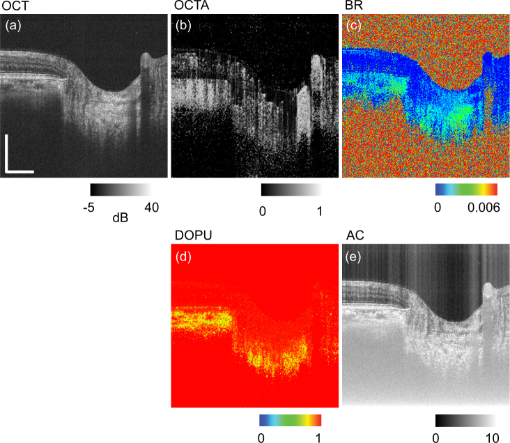
The JM-OCT system multiplexes images that correspond to two incident polarization states at two depths, and simultaneously measures two spectral interferograms using a polarization diversity detector. Thus, the JM-OCT data consist of four OCT images that could be combined to obtain functional contrasts, including scattering intensity (OCT), OCT angiography (OCTA), degree of polarization uniformity (DOPU), local birefringence (BR) and attenuation coefficient (AC). In addition, frame (B-scan) acquisition is repeated four times at the same position on the retina.

The scattering intensity OCT was computed from the set of four OCT images of a Jones matrix as follows. First, two images of the same detection channel are combined coherently by a coherent composition method [10]. It gives complex OCT images corresponding to two detection polarization channels. And for each channel, four repeating frame images were obtained. The images were converted into squared intensity, the four repeating frames are averaged in intensity, and the averaged intensity images of two detection polarization channels were summed. This process finally gives polarization artifact-free OCT intensity tomographies.

OCTA was obtained using complex correlation analysis with Makita’s noise-correction [12] among the four repeated frames.

BR was computed using a local Jones matrix analysis method [34] and maximum a-posteriori (MAP) BR estimator [35]. Before applying the MAP BR estimator, the four repeated frames, i.e., four Jones matrices, were combined by adaptive Jones matrix averaging method [9, 10]. The local Jones matrix analysis was applied with 6-pixel depth separation (24-µm) and the MAP estimation was performed with a spatial kernel of 2 pixels (42 µm, lateral) × 2 pixels (8 µm, depth).

DOPU was computed over a spatial kernel of 3 × 3 pixels over four repeated frames and two input polarizations with noise correction [13].

AC was computed using a model-based reconstruction method presented by Vermeer et al. [36] with modification for polarization diversity detection [37]. Specifically, we used Eq. (14) in Ref. [37] for the AC computation where OCT intensity, I(z_i), was the above mentioned polarization artifact-free OCT intensity (Eq. (9) in Ref. [37]). We omitted the signal roll off correction for this AC computation because the signal roll off appeared as a nearly constant bias of the AC and did not affect the subsequent tissue classification.

More details of JMOCT-related signal processing are summarized in Refs. [10,11]. An example set of cross-sectional ONH images of the above five contrasts are shown in Fig. 1 as follows: (a) OCT, (b) OCTA, (c) BR, (d) DOPU, and (e) AC.

Fig. 1.

Example of multiple contrasts of an ONH cross-section obtained by JM-OCT: (a) OCT intensity (OCT), (b) OCT angiography (OCTA), (c) birefringence (BR), (d) degree of polarization uniformity (DOPU), and (e) attenuation coefficient (AC). Scale bars indicate 0.5 mm × 0.5 mm.

2.2. The tissue classification framework

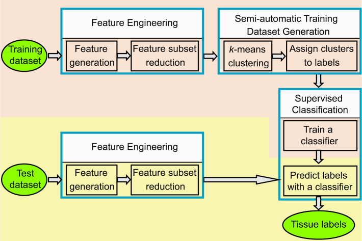
The tissue classification framework used in this study consists of four phases: feature engineering, semi-automatic generation of training dataset, supervised training of tissue classifier, and tissue classification by the trained classifier. This framework is summarized in Fig. 2. The entire framework was run on two disjoint subset of data: one for training and the other for classification testing. Each of these phases is discussed in detail in the following.

Fig. 2.

The framework of our tissue classification method. It consists of training set generation (pink region) and classification process (yellow region). The circle and rectangle objects represent the data and the operations, respectively.

2.2.1. Feature engineering

The steps to create new feature set, which is going to be used for tissue classification, from the raw JM-OCT contrasts (primary features) are described in this section. Throughout the remainder of the paper, M represents the number of features, i.e., the dimensions of the feature space. The subscript with M denotes whether the feature set is primary (p), extended (ext) or reduced (r), as explained later in this section. Each of the features is represented by X_i, where i varies from 1 to M. Feature engineering consists of two steps; the generation of extended feature set and subsequent reduction.

In the extended feature generation process, the five primary features (M_p = 5) including OCT, OCTA, BR, DOPU, and AC, are extend into a M_ext = 16 features. The extended feature set includes OCT, OCTA, BR, DOPU, AC, OCT × (1-DOPU) × OCTA, AC × (1-DOPU) × OCTA, OCT × BR, AC × BR, AC × DOPU, AC × OCTA, DOPU × OCTA, BR × DOPU, OCTA/AC, OCT/AC, and OCT ⊕ AC. Among the extended features, OCT, OCTA, BR, DOPU, and AC are direct copies of the primary features. OCT × (1-DOPU) × OCTA and AC × (1-DOPU) × OCTA are expected to be sensitive to a hyper-scattering, melanin-containing, and vascular rich tissue. OCT × BR and AC × BR become large for hyper-scattering and highly birefringent tissues, such as collagen-rich tissue. AC × DOPU is expected to be sensitive to hyper-scattering and less-melanin tissues. Because hyper-scattering tissues, such as RPE and choroid, contain melanin, this feature is expected to distinguish less-melanin high-density tissues from melanin-rich high density tissues. AC × OCTA and DOPU × OCTA are expected to be sensitive to highly vascular tissue. BR × DOPU is included to be sensitive to less-melanin fibrotic tissues, such as nerve fibers and/or collagen. OCTA/AC and OCT/AC are included to separate vessels and their shadow. OCT ⊕ AC is a bit-wise exclusive OR (XOR) operation where OCT are in dB scale and both OCT and AC are in unsigned 8-bit integer representation. Although the physical interpretation of this feature is not fully clear, it was included in order to highlight the difference between OCT and AC. The rationality of this feature is further discussed in Section 4.1. Each feature is then rescaled using z-score normalization [38] so that it has a zero mean and an unit variance.

The extended feature set is then truncated by removing redundant features. The Pearson’s correlation coefficients of all pairs of features are computed. If the correlation coefficients of a particular feature pair exceed 0.95, then one of the feature of the pair is eliminated. If one of the feature in the correlated pair is a primary feature, then the other is eliminated. In our particular research on ONH, this process eliminated four features: AC × BR, which correlated with BR (ρ = 0.971); AC × OCTA, which correlated with OCTA (ρ = 0.973); DOPU × OCTA, which correlated with OCTA (ρ = 0.996); and BR × DOPU, which correlated with BR (ρ = 0.997). Thus, the size of the reduced feature set was M_r = 12 and it included OCT, OCTA, BR, DOPU, AC, OCT × (1-DOPU) × OCTA, AC × (1-DOPU) × OCTA, OCT × BR, AC × DOPU, OCTA/AC, OCT/AC, and OCT ⊕ AC. This feature reduction reduces the dimension of the feature space used in the subsequent processes including the generation of training dataset, which is based on k-means clustering, classifier training, and final tissue classification. Thus, it reduces the processing time of these processes.

2.2.2. Semi-automatic generation of training dataset

In our segmentation framework, the training dataset used for subsequent training of a random forest classifier is semi-automatically generated. This process consists of two main steps: an unsupervised method for clustering in M_r-dimensional feature space and manual interpretation of the clusters that assign particular tissue labels to each cluster. The details are as follows.

The first step involves pixel-by-pixel clustering in the M_r-dimensional feature space, which is 12-dimensional in our particular case. Clustering is performed by k-means clustering algorithm. To make clustering meaningful, the number of clusters (k) should be larger than the number of tissue types in the image. By contrast, too many clusters makes the subsequent manual interpretation difficult and time-consuming. In our particular implementation, k = 72 was empirically chosen. Clustering was performed over a maximum of 300 iterations for a single trial. Ten trials were performed with different initial distributions of clusters (seeds), and the best results were selected as the final clustering result. The goodness of each trial was assessed by computing a metric so called as “inertia,” which is the summation of squared distances from each pixel to the centroid of the corresponding cluster in M_r-dimensional feature space. The k-means clustering algorithm was implemented using the machine learning library scikit-learn 0.18 on Python 2.7.

In the second step, a particular tissue label was manually assigned to each cluster. For this manual tissue label assignment, the pixels of each cluster were overlaid on the OCT image, and an expert grader (DK) reviewed this OCT image and assigned a proper tissue label based on anatomical knowledge [39, 40]. This two-step process dramatically reduced the effort of the training dataset generation process in comparison to a standard method, which involves fully manual segmentation of multiple tissue types, as discussed in Section 4.5.

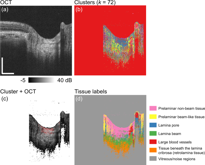
Figure 3 exemplifies the training dataset generation process. Figure 3(a) is an example of the OCT image. In our particular implementation for ONH analysis, only the region within the optic disc was used (see Section 2.3.2 for details). Fig. 3(b) shows all 72 clusters, where each cluster is displayed with each randomly selected color. Fig. 3(c) shows the manual tissue label assignment process, where pixels that belong to one of the clusters are highlighted in red and overlaid on the OCT image. The expert grader selected one of the most suitable tissue labels (classes) for the cluster. In our particular ONH implementation, there were seven tissue labels (classes) (see Section 2.3 for details). This process was performed for all the k = 72 clusters. Fig. 3(d) shows the distributions of the tissue labels, where each label is displayed with each random color.

Fig. 3.

Example of manual tissue label assignment: (a) an OCT image, (b) clusters with each different color, (c) example of a cluster (red) overlaid on the OCT, (d) tissue labels as each label is displayed with each color. Scale bars indicate 0.5 mm × 0.5 mm.

2.2.3. Supervised classification

The third step is training of the multi-class classifier using the generated training dataset. In our particular implementation, the classifier was a random forest classifier. The random forest consisted of 10 decision trees. The quality of the tree-node split was defined using the Gini impurity. The maximum number of features, based on which the split was chosen, was $\sqrt{M_r}$, and the maximum depth of a tree was 20. Each tree was trained using a randomly selected subset of pixels by following the standard training method of a random forest classifier. The random forest classifier was implemented using the same library as k-means clustering (scikit-learn 0.18 on Python 2.7).

In the final step, each pixel in the test dataset was classified into one of the tissue classes using the trained classifier.

2.3. ONH analysis

The tissue classification framework discussed in the previous section is a general framework and it could be customized to several types of JM-OCT images, such as anterior eye [29,30], posterior eye [11, 41, 42], heart [43], and skin [44]. In this study, we specialized the algorithm for the classification of lamina cribrosa and its surrounding tissues in the ONH region. Particularly, the primary focus was to segment the lamina beam for 3-D morphological and functional assessment.

2.3.1. Measurement protocol and the subjects

Six eyes of three Asian subjects, including normal and myopic cases, were imaged for the study. A 3 mm × 3 mm area around the ONH was scanned using a horizontal fast raster scan protocol, which consisted of 512 Alines/B-scan times 256 B-scans times 4 repeats at each B-scan location. Each volume acquisition took approximately 6.6 seconds.

The biometric parameters including refractive error, axial eye length (AL), and intraocular pressure (IOP) were measured using RT-7000 (Tomey Corp.), IOL Master (Carl Zeiss), and Goldmann applanation tonometer, respectively. The biometric measurement was performed within an hour of the OCT imaging session by experienced ophthalmologists at the University of Tsukuba.

The mean age of the subjects was 42.5 ± 11.5 years (mean ± standard deviation; range: 30.4 to 56 years old). A JM-OCT volume was obtained for each eye, so six volumes were obtained from the three subjects in total. The right eyes were used for the training dataset and the left eyes were used for the test dataset. The details of the subjects used in the study are summarized in Table 1.

Table 1.

Subject details and the biometrics of the subjects. SE, AL, and IOP are for spherical equivalent refractive error, axial eye length, and intraocular pressure, respectively. Subjects-1 and 2 are regarded as myopic in this study, while Subject-3 is regarded as emmetropic.

Subject ID	Age (y/o)	Sex	Eye	SE (D)	AL (mm)	IOP (mmHg)	Usage
Subject-1	41.2	M	R	−7.50	27.12	17	Training
			L	−7.25	27.0	16	Test
Subject-2	56.0	M	R	−8.00	27.38	17	Training
			L	−7.75	26.74	18	Test
Subject-3	30.4	F	R	−0.50	23.72	14	Training
			L	−0.25	23.62	14	Test

The study protocol adhered to the tenets of the Declaration of Helsinki, and was approved by the Institutional Review Board of the University of Tsukuba.

2.3.2. Preprocessing, tissue classification, and post-processing for the ONH dataset

The following preprocessing was performed to reduce the number of pixels in the training dataset and hence, reduce the training time. First, the OCT-intensity-based threshold was applied to remove very low intensity (noise) pixels from the training dataset. The threshold was applied after two-dimensional median filtering (3 pixels (lateral) × 3 pixels (axial) kernel over the B-scan). Second, for each of the training dataset volumes, only three B-scans each per volume was randomly selected to reduce the size of the training dataset. Thus, nine B-scans of three right-eye volumes from three subjects were jointly used as the input to k-means clustering, and hence used as the training dataset.

Third, a manual delineation of the optic disc was performed to use only the optic disc region for training. The manual delineation was performed by an expert (DK) by detecting the limit of the Bruch’s membrane in the OCT images. The OCT-intensity-based threshold was applied to both training and test data, whereas the delineation of the optic disc was performed only for training data. Thus, tissue classification was performed not only on the pixels within the optic disc, but also on the pixels outside the optic disc. Although the classification were performed for the entire volume of the test dataset, only the tissue labels obtained within the optic disc were considered meaningful and worth further interpretation.

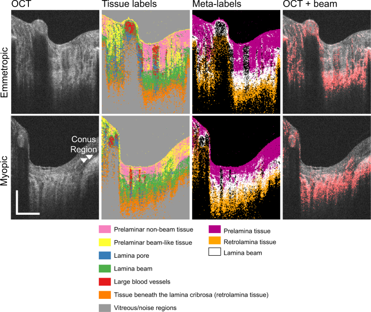
k-means clustering for the training dataset generation and the random forest classifier were implemented using the Python-based machine learning library scikit-learn 0.18 on Python 2.7. Python libraries for numerical computation, Numpy 1.11 and Scipy 0.19, were additionally used. Processing was performed on a CPU (non-GPU) environment on Windows 10. The classifier was trained to classify each pixel into one of seven tissue classes: prelaminar beam-like tissue, prelaminar non-beam tissue, lamina beam, lamina pore, tissue beneath the lamina cribrosa (retrolamina tissue), large blood vessels, and vitreous/noise region. Three meta-labels are then obtained from the classified tissue labels. The meta-label of prelamina tissue is the combination of prelamina beam-like and prelamina non-beam tissue labels. The meta-labels of the lamina beam and retrolamina are identical to the classification labels of lamina beam and retrolamina tissues, respectively. In this particular study, the tissue of main focus was the lamina beam.

Before further analyzing the lamina property using the classification result, inter-frame motion was corrected using the Register Virtual Stack Slices plugin and Transform Virtual Stack Slices plugin on an open-source image processing platform Fiji [45], where the motion was detected from the OCT intensity volume, and the motion in all types of the volumes were corrected by the detected motion. For en face visualizations in Section 3, the optic disc was manually defined by looking at the OCT projection image over the entire depth, and its best fit ellipse was drawn as a region-of-interest (ROI). The myopic conus region were excluded from the ROI.

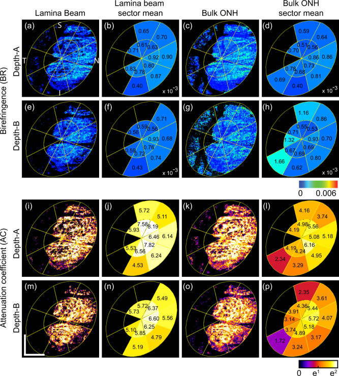
We used the segmented lamina beam as a 3-D mask to obtain the lamina beam birefringence and attenuation coefficient maps, where the birefringence and attenuation coefficient were the BR and AC data of the same JM-OCT volume. The lamina beam maps were further sectorized. The sectors were defined within the elliptic ROI. The ellipse was first split into two concentric ellipses. The long and short diameter of the smaller ellipse were half the respective diameters of the larger ellipse. Each ellipse was further split into eight equi-angle radial pieces; thus, we finally had 16 sectors, as later shown in Figs. 9 and 10. The mean birefringence was computed for each sector within a thin depth region of 5 pixels. For comparison, a sectorized mean birefringence map of bulk ONH was also created. To exclude blood vessels, a 3-D binary mask was created by applying the moments binarization method [46] (Fiji standard implementation) to the full-depth OCT volume. The mean attenuation was computed for each sector within the depth region of 5 pixels. The averaging of attenuation was performed on a linear scale; however, color representation is on a logarithmic scale. For bulk ONH attenuation coefficient maps were also computed. For bulk ONH maps, blood vessels were excluded using the same mask applied to the bulk ONH birefringence maps.

Fig. 9.

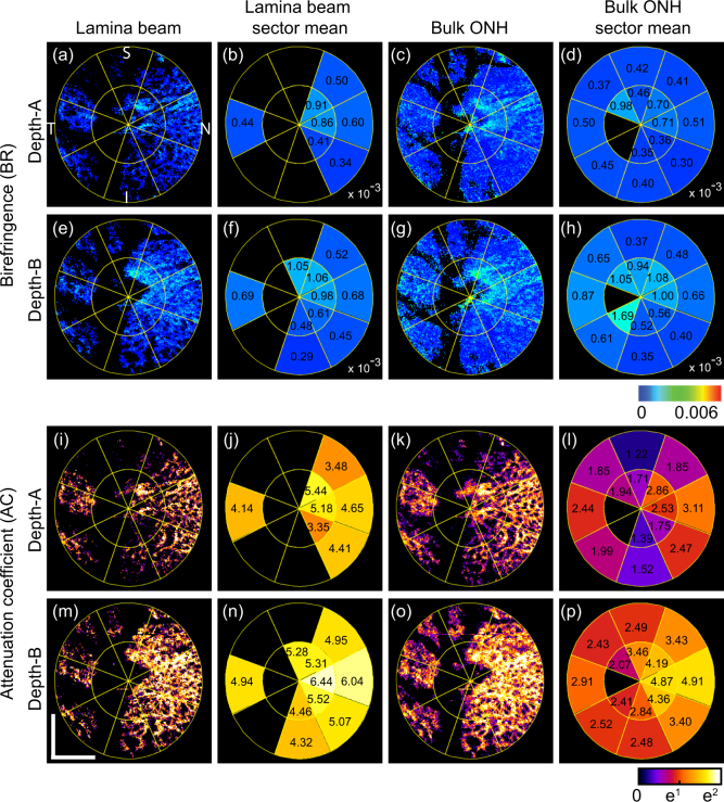
En face birefringence maps (first and second rows) and attenuation coefficient maps (third and fourth rows) for the emmetropic case (Subject-3) that corresponds to Fig. 5. The first and the third rows correspond to depth-A, while the second and the fourth rows correspond to depth-B as shown in Fig. 5(a). (a) and (e) are en face lamina beam birefringence, where the non-lamina beam tissues were masked out by using the segmented lamina beam. (b) and (f) are sectorized birefringence maps of the lamina beam. (c) and (g) are bulk ONH birefringence, while (d) and (h) are sectorized birefringence maps of the bulk ONH. (i) and (m) are en face lamina beam attenuation coefficient. (j) and (n) are sectorized attenuation coefficient maps of the lamina beam. (k) and (o) are bulk ONH attenuation coefficient, while (l) and (p) are sectorized attenuation coefficient maps of the bulk ONH. Scale bars indicate 0. 5 mm × 0.5 mm.

Fig. 10.

En face birefringence maps (first and second rows) and attenuation coefficient maps (third and fourth rows) for the myopic case (Subject-1) that corresponds to Fig. 6. Subfigure configuration is identical to Fig. 9. Scale bars indicate 0. 5 mm × 0.5 mm.

For comparison, the sectorized mean birefringence and attenuation coefficient maps of lamina pore were obtained. The lamina pore region is defined as non-lamina-beam and non-blood vessel pixels within the bulk lamina region. It should be noted that this lamina pore is not identical to the tissue label of the lamina pore described in Section 2.3.2. Quadrant sectors (temporal, superior, nasal, and inferior) were used for simplicity of comparison rather than the 16 sectors.

3. Results

3.1. Tissue segmentations

Figure 4 shows examples of ONH tissue classification results as cross-sectional images, where only the regions within the optic disc are shown. The first and the second rows show the cases of emmetropia (left eye of Subject-3) and myopia (left eye of Subject-1), respectively. The first column shows the OCT images. The second column shows the output of the classifier, that is, the tissue label images, where each tissue type (label) is shown in a different color. The third column shows the “meta-label” images, where each meta-label is a combination of classified tissue labels. In the tissue label and meta-label images, the boundary of lamina cribrosa and retrolamina tissues is relatively poorly delineated, whereas the junction between the prelamina tissue and lamina cribrosa shows relatively sharp appearance. This agrees with histological knowledge, that is, lamina-cribrosa-to-retrolamina transition is moderate, whereas that between the prelamina and lamina cribrosa is sharp [47]. The fourth column shows the OCT cross-section, where the lamina beam pixels are highlighted in red. The segmented lamina beam pixels are well co-registered with the lamina beam appearances in the OCT intensity images. This agreement between the segmented lamina beam and OCT intensity is more clearly shown in the en face images in Figs. 5 and 6.

Fig. 4.

Examples of tissue classification results. First and second rows are for an emmetropic case (left eye of Subject-3) and a myopic case (left eye of Subject-1), respectively. Each column, from left to right, represents the images: OCT, tissue labels, meta-labels, and lamina beam pixels (red) overlaid on the OCT. Meta-labels are for prelamina tissue, lamina beam, and retrolamina tissue. Scale bars indicate 0.5 mm × 0.5 mm.

Fig. 5.

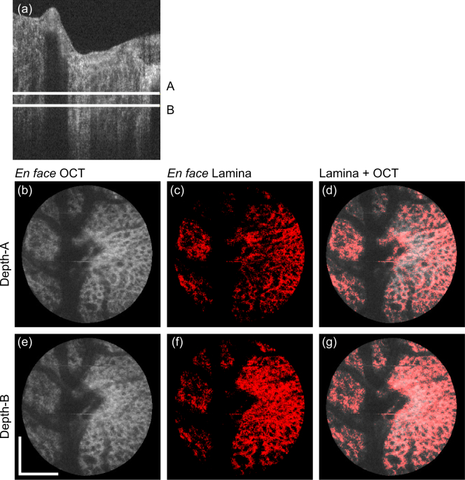
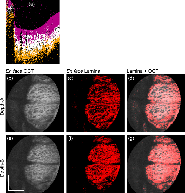
En face projection images of the emmetropic case that corresponds to the first row of Fig. 4. (a) Representative B-scan, where two depth positions (A and B) are indicated. (b)–(d) and (e)–(g) are en face slices obtained at the depth-A and depth-B, respectively. (b) and (e) are the OCT intensity, (c) and (f) are the segmented lamina beam, and (d) and (g) are the OCT intensity on which the lamina beam pixels are overlaid in red. Scale bars indicate 0. 5 mm × 0.5 mm.

Fig. 6.

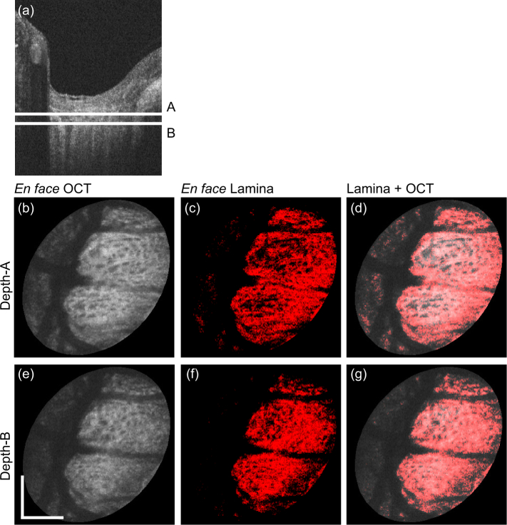
En face projection images of the myopic case that corresponds to the second row of Fig. 4. Subfigure configuration is identical to Fig. 5. Scale bars indicate 0.5 mm × 0.5 mm.

The entire B-scans of the same volumes in Fig. 4 are processed by the same trained classifier, and en face lamina beam images were created. Figures 5 and 6 show the emmetropic (left eye of Subject-3) and myopic (left eye of Subject-1) cases that correspond to the first and second rows of Fig. 4, respectively. Figures 5(a) and 6(a) are representative of the cross-sectional OCT, where two depth positions (A and B) are indicated by white horizontal lines. Figures 5(b)–(d) and 6(b)–(d) are en face slices at depth-A, whereas Figs. 5(e)–(g) and 6(e)–(g) are at depth-B. Figures 5(b), 5(e), 6(b), and 6(e) are the OCT intensity slice, which are depth-averages of 5-pixel-depth slabs centered at depths A and B, respectively. Figures 5(c), 5(f), 6(c), and 6(f) are the en face segmented lamina-beam images at the depths A and B, respectively. These en face images are also the depth average of 5-pixel-depth, and the averaging was performed as the lamina beam pixels as 1.0 and other pixels as 0.0. Figures 5(d), 5(g), 6(d), and 6(g) are the segmented lamina beam (red) overlaid on the OCT intensity slice. The en face images show a clearer contrast of the meshwork structure of the lamina beam than the cross-sectional images. Particularly in the emmetropic case (Fig. 5), the depth wise difference of the lamina beam pattern is clearly shown.

3.2. Comparison with manual segmentation

The accuracy of the segmentation results was examined by comparing the results obtained from manual segmentation. Manual segmentation was performed for a cross-sectional image and two en face sections per subject. The cross-section and en face slices were the same as those shown in Figs. 4, 5 and 6. For the cross-sectional image, an expert manually traced the boundary among the prelamina, lamina cribrosa and retrolamina regions by looking at the OCT intensity image. For the en face slices, the lamina pore and noise regions were manually highlighted and then the segmented region was inverted to highlight the lamina beam; that is, the lamina beam region was segmented as non-lamina-pore and non-noise regions. The agreement between manual and automatic segmentation was evaluated using Dice coefficients.

The computed Dice coefficients of the pre-lamina tissue in the cross-section were 0.55, 0.53, and 0.50 for Subjects-1, 2, and 3, respectively. Those for the retrolamina tissue were 0.45, 0.13, and 0.31 for Subjects-1, 2, and 3, respectively. The Dice coefficients of the lamina beam were 0.79 and 0.77 for Subject-1, 0.78 and 0.79 for Subject-2, and 0.55 and 0.69 for Subject-3. The two Dice coefficients of each subject correspond to Depths A and B, respectively.

For lamina beam tissue, moderate to high Dice coefficients, that is, moderate to high agreement between manual and automatic segmentation, were found. By contrast, the Dice coefficients of pre-lamina and retrolamina tissues were not high. The relatively low Dice coefficients can be partially accounted for by non-perfect manual segmentation and a difference in the definition of the tissue regions between manual and automatic segmentation. For example, the lamina pore and lamina beam in the cross-sectional scattering OCT were also difficult to manually delineate. Hence, we delineated lamina-to-pre-lamina and lamina-to-retrolamina interfaces rather than segmenting each lamina beam. This resulted in an evident shortcoming such that the lamina pore regions were not classified as pre-lamina or retrolamina regions using manual segmentation, whereas they were classified as either pre-lamina or retrolamina regions using automatic segmentation. In addition, the boundary between lamina cribrosa and retrolamina tissues is anatomically not sharp [47]. Thus, manual delineation of the lamina-retrolamina boundary is inevitably not perfect. Manual segmentation for a lamina beam in en face slice is also not fully reliable; because of its low intensity contrast and limited transversal resolution of OCT.

3.3. Effect of correlation between the test and training datasets

In our main result in Section 3.1, we used the collateral eyes of the same subjects to train the classifier (with right eyes) and validate the classifier (with left eyes). Although the training and validation were performed using different eyes, the eyes from the same subjects might have some correlation. To evaluate the effect of the collateral correlation, we trained the classifier using the right eyes of two of the three subjects, and examined the classifier using the left and right eyes of the residual subject. Thus, it is a leave-one-out validation.

Because all six trials demonstrated similar results, two representatives are shown in Fig. 7. The upper half of the figure shows images of the left eye of Subject-3 (emmetropia), whereas the lower half shows the left eye of Subject-1 (myopia). The first column shows the original segmentation results which are identical to Figs. 4, 5 (c), 5 (f), 6 (c), and 6 (f). The second column shows the results that correspond to the first column but were obtained using leave-one-out validation. The third column shows the red-green composite of the en face segmentation results, where the original and leave-one-out segmentation results are in red and green, respectively. The overlapping pixels of the two segmentation appears in yellow. The first and fourth rows show cross-sectional meta-label images, the second and fifth rows show the en face lamina beam at Depth-A, and the third and sixth rows show that at Depth-B. The depths are indicated in Figs. 5 and 6.

Fig. 7.

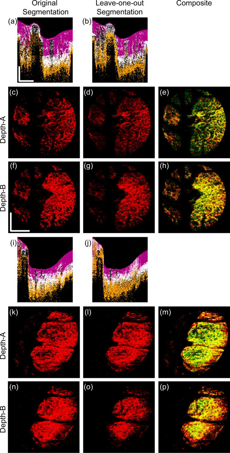
A comparison of the original and leave-one-out segmentations. The upper half of the figure shows the images of the left eye of Subject-3 (emmetropia); and the lower half shows the left eye of Subject-1 (myopia). The first and second columns show the original and leave-one-out segmentations. The third column shows the red-green composite of the first and second column images, where the original and leave-one-out segmentation results are in red and green, respectively. The first and fourth rows show the cross-sectional meta-label images, the second and fifth rows show the en face lamina beam at Depth-A, and the third and sixth rows show that at Depth-B. Scale bars indicate 0.5 mm × 0.5 mm.

Although some minor discrepancies were found in the low intensity region and periphery, the original and leave-one-out segmentations of the lamina beam agreed reasonably.

3.4. Long-term robustness of the classifier

To test the long-term robustness of the trained classifier, the classifier trained in Section 3.1 for Figs. 5 and 6 was applied to the another dataset of Subject-1 that was acquired 6 months after the acquisition of the training dataset.

The results are summarized in Fig. 8. Figure 8(a) shows the cross-sectional meta-label image, and the alignment of en face images [Figs. 8(b)–(g)] is the same as the corresponding original segmentation results at the baseline time point [Fig. 6]. By comparing this result of after 6 months with the baseline result, a high consistency is seen in the segmentation results. This demonstrates the reasonable long-term robustness of our method.

Fig. 8.

Segmentation results of the myopic eye (Subject-1). Segmentation was performed using the same trained classifier as Fig. 6 however, the data were acquired 6 months after the training dataset was acquired. (a) represents the cross-sectional image of the meta-labels. The alignment of (b)–(g) was identical to that of Fig. 6. Scale bars indicate 0.5 mm × 0.5 mm.

3.5. Lamina beam birefringence and attenuation coefficient analysis

The lamina beam and lamina pore are two distinguished tissues. The lamina beam consists of collagen and its ultrastructure supports the mechanical characteristic of the lamina cribrosa. Hence, the birefringence and scattering characteristic analysis of only lamina beam regions can be more sensitive to pathologic tissue alteration than the analysis of the entire lamina cribrosa. The lamina beam segmentation described in this paper allows us to specifically assess the optical properties of the lamina beam.

Figures 9 and 10 show the lamina beam birefringence and attenuation coefficient maps of emmetropic (left eye of Subject-3) and myopic (left eye of Subject-1) cases, respectively. The first two rows are birefringence maps, while the third and fourth rows are attenuation coefficient maps. The first to last columns of the figures are en face slices of lamina beam birefringence/attenuation coefficient (first column), sectorized mean birefringence/attenuation coefficient of lamina beam (second column), bulk lamina birefringence/attenuation coefficient (third column), and the sectorized mean birefringence/attenuation coefficient of bulk ONH (fourth column). The first and third rows of both figures correspond to depth-A of Figs. 5 and 6, whereas the second and fourth rows correspond to depth-B. The sector borders are overlaid on the maps.

In the mean lamina beam birefringence maps [Figs. 9(b), 9(f), 10(b), and 10(f)], the inter-sector difference is clear. In depth-A of both cases, the beam birefringence is generally higher than the bulk ONH birefringence. In depth-B, the mean birefringence values of the beam and bulk ONH are more similar than the depth-A. It would be explained by the higher density of beam at depth-B than depth-A.

In the attenuation maps, significantly higher sectorized mean attenuation can be found in lamina beam attenuation maps than the bulk ONH attenuation maps at both depths and both cases. It is also because of the contribution of low scattering non-beam tissue in the bulk ONH attenuation maps.

Because the beam birefringence and attenuation coefficient maps reflect only the beam property, it would be more sensitive to the tissue alteration of the lamina cribrosa. Thus, it could be useful for the detection of early pathologic alteration.

The mean birefringence and attenuation coefficients of the lamina-beam and lamina pore regions in the quadrant sectors are summarized in Table 2, where the upper values in each cell are for the lamina beam and the lower values in brackets are for the lamina pore. For all sectors of both depths, the mean attenuation coefficients of the lamina beam were found to be higher than those of the lamina pore. For six out of 16 combinations of sectors and depths, the mean birefringence of the lamina beam was found to be higher than those of the lamina pore. This contradicts our initial expectation that the lamina beam would generally have higher birefringence than the lamina pore. However, it is consistent with the fact that birefringence had relatively low feature importance for the classification as later discussed in Section 4.2.

Table 2.

Sector-wise mean values of birefringence and the attenuation coefficient. The values outside and inside the brackets represent the lamina-beam and non-lamina beam, respectively. Values in red indicate the region in which lamina beam values are higher than non-lamina beam values.

		Birefringence (× 10−3)				Attenuation coefficient (mm−1)
		Temporal	Superior	Nasal	Inferior	Temporal	Superior	Nasal	Inferior
Subject-3 Emmetropia	Depth-A	0.40	0.38	0.63	0.33	4.00	3.29	4.36	3.98
		(0.55)	(0.46)	(0.47)	(0.35)	(1.51)	(1.29)	(1.43)	(1.28)
	Depth-B	0.63	0.56	0.71	0.45	4.89	4.56	5.66	4.95
		(0.87)	(0.59)	(0.63)	(0.40)	(1.95)	(1.86)	(2.16)	(1.89)
Subject-1 Myopia	Depth-A	0.73	0.66	0.87	0.61	5.14	5.97	6.52	5.14
		(0.95)	(0.53)	(0.71)	(0.55)	(2.05)	(2.55)	(2.62)	(2.03)
	Depth-B	0.63	0.68	0.77	0.57	6.00	5.62	5.68	5.51
		(1.88)	(0.94)	(0.78)	(0.99)	(1.72)	(2.08)	(1.98)	(1.78)

4. Discussions

4.1. Rationality of XOR feature

Bit-wise XOR of OCT and AC (OCT-⊕-AC) has been used as a feature in the present tissue classification method. This feature was introduced as one of the extended features and also was retained in the reduced feature. So it was used for the tissue classification by the random-forest classifier.

Although the physical interpretation of this feature is still an open issue, it was found that this feature positively affects the lamina beam segmentation. This positive effect was shown by the following two findings.

The first finding is that OCT-⊕-AC showed 5th highest feature importance among the twelve reduced features. Here, the feature importance was Gini importance [48] and was obtained as a built-in attribute of the sci-kit learn implementation of the random-forest classifier.

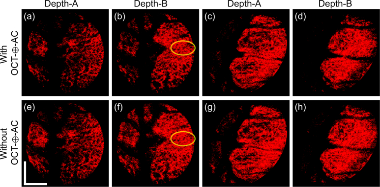
The second finding is shown in the comparison of lamina beam segmentation results obtained with and without OCT-⊕-AC feature (Fig. 11). The upper row [Figs. 11(a)–(d)] are segmented lamina beam with the OCT-⊕-AC feature, which are identical to Figs. 5(c), 5(f), 6(c), and 6(f), respectively. The lower row [Figs. 11(e)–(h)] are the same segmentation results but obtained without the OCT-⊕-AC feature. The images were obtained at two depths [depths A and B indicated in Figs. 5(a) and 6(a)]. The left four and right four images were obtained from the emmetropic subject (Subject-3) and the myopic subject (Subject-1), respectively. It is seen that the segmentation results with the OCT-⊕-AC feature shows clearer structure of lamina pores than that without the OCT-⊕-AC feature as exemplified by yellow circles. These two findings support the inclusion of this feature.

Fig. 11.

The comparison of lamina beam segmentation results with and without OCT-⊕-AC feature. (a)–(d) are segmented lamina beam with the OCT-⊕-AC feature, while (e)–(h) are without the OCT-⊕-AC feature. The images are obtained at two depths as indicated in the figure The left four images (a), (b), (e), and (f) are from the emmetropic subject (Subject-3) and right four images (c), (d), (g), and (h) are from the myopic subject (Subject-1). (a)–(d) are identical to Figs. 5(c), 5(f), 6(c), and 6(f), respectively.

There must be other synthesized features which do not have straight physical interpretation but are still useful for tissue classification. Usage of standard machine learning techniques will enable the usage of such features. For example, a neural network based auto-encoder can generate new synthesized features without considering its physical interpretations (see also Section 4.4). A support vector machine classifier also generates high-order features by itself owing to its kernel methods.

4.2. Features and classification

The trained random forest algorithm provided the importance metric (Gini importance [48]) for each feature. Figure 12 shows the mean feature importance and its standard deviation over the 10 decision trees used in our trained random forest classifier. AC × (1-DOPU) × OCTA and OCT × (1-DOPU) × OCTA were the top two features with the highest mean feature importance. It can also be seen that the AC and features associated with AC seems to play a major role in the classification, followed by OCT, OCTA, DOPU and BR, in that order. It is also seen in the results shown in Section 3.5 that the mean AC values showed an evident difference between lamina and non-lamina tissues, while the difference was not clear in BR.

Fig. 12.

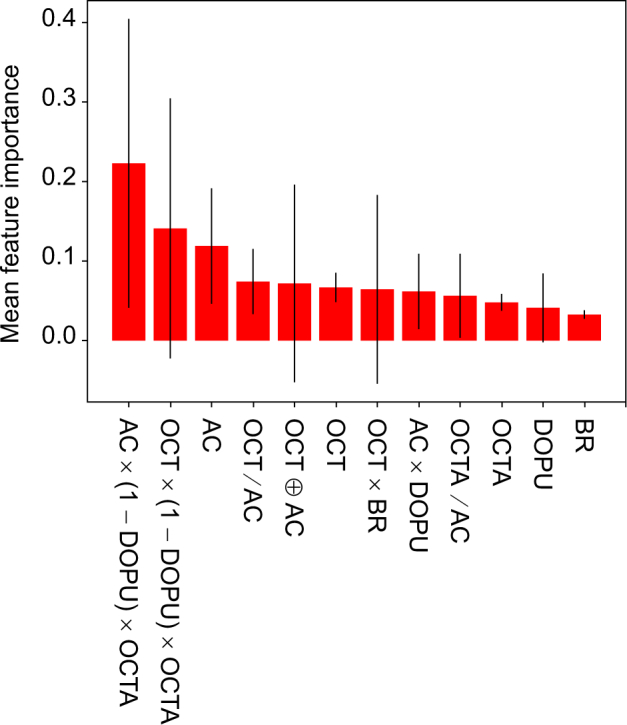
The mean and standard deviations of the Gini importance for each feature. The mean was computed over 10 decision trees in the trained random forest classifier. The heights of the red bars indicate the mean importance of each feature; and the black lines indicate the standard deviation.

Azuma et al. recently demonstrated a generation of features by combining multiple contrasts of JM-OCT [25], and the features are sensitive for specific tissues. The feature specific to RPE was AC × (1 − DOPU) × (1 − OCTA_b) where OCTA_b is a binarized OCTA. It is noteworthy that this RPE feature is similar to the 1st important feature and it can be generated by combining our 1st, 3rd and 8th important features, although the OCTA used in our study was not binarized.

4.3. Potential clinical applications

Glaucoma and myopia are known to be associated with ONH alterations [49–51]. Particularly, glaucoma is believed to show ultrastructural alterations in its very early stage, even before the thinning of retinal nerve fiber layer [52].

Our method enables the specific investigation of only the lamina beam as demonstrated in Section 3.5. Not only birefringence analysis, but also the lamina beam segmentation result can be used to analyze other optical properties. For example, the attenuation coefficient is also expected to be an early biomarker of glaucoma [36,53]. The attenuation coefficient assessment specific to the lamina beam may also be useful for glaucoma detection.

4.4. Potential usage of other machine learning algorithms

In the current method, we first expanded the feature space from M_p (= 5) to M_ext (= 16) by combining the original optical features. Then, it was reduced by checking the correlation among the extended features. Although this empirical feature engineering was satisfactory for our specific purpose, it would be good if this feature engineering was not empirical so as to generalize our tissue classification framework to the other types of tissues. Neural network-based auto-encoders can potentially be used for the non-empirical feature engineering.

In the current method, we used a random forest classifier. However, other classifiers, such as support vector machines, can also be used. Although the current random forest classifier was satisfactory for our specific purpose, there is still scope for optimization, particularly for tailoring the method to other tissue types.

4.5. Processing time

The processing time could be calculated as the total time involved in the entire processing, including the training and testing phases. Broadly, it can be divided into processing the JMOCT contrasts for feature engineering, generation of the training dataset, and predicting tissue labels on the test data.

The first stage was data preparation, including JM-OCT image construction, general post-processing, and feature engineering. The generation of five primary contrasts and feature engineering took approximately 35 minutes for a single volume.

The second stage was the training stage, which involved the unsupervised learning stage of k-means clustering and the manual process of assigning the clusters to pre-assigned tissue labels. k-means clustering over three B-scans of 512 × 500 for three volumes took approximately 11.4 minutes. The manual cluster assignment took another 10 minutes, and training this dataset with the random forest classifier took 17.4 seconds. In total, approximately 22 minutes was required for the generation of the training dataset using the random forest classifier.

The third stage was the supervised classification of each volume dataset. It took approximately 25 seconds to predict the tissue labels over the entire volume of test dataset of 512 × 500 × 256 pixels.

The implementation was run on a Windows 10 PC with Intel (R) Core (TM) i9-7900X CPU (3.30GHz) and 128 GB RAM.

4.6. Limitations of the present method

Although reasonable segmentation results were demonstrated for a single myopic case and a single emmetropic case, the present method still has some limitations.

Although the method was described as pixel-by-pixel classification, some of the JM-OCT contrasts were computed using spatial kernels. For example, OCTA and DOPU were computed using a spatial kernel of 3 × 3 pixels (lateral × axial; 63 µm × 12 µm). BR was computed from two pixels with 6-pixel (24-µm) depth separation, and then a MAP birefringence estimator [35] was applied with a spatial kernel of 2 × 2 pixels (lateral × axial; 42 µm × 12 µm). Thus, the resolution of the segmentation was limited by the sizes of the kernels and it may have reduced the contrasts of the OCTA, DOPU, and BR images.

In the present study, the size and variability of the training and test datasets were limited. The versatility of the segmentation method should be evaluated with larger and more varied datasets.

The current algorithm still exhibits some evident misclassification. For example, as seen in the meta-labels of Fig. 4, the walls of some large blood vessels are misclassified as lamina beam. Also, most of the pixels in the shadow of the large blood vessels are misclassified as retrolamina pixels. So, the interpretation of segmentation results around the large blood vessels should be done with care. Although our current algorithm was designed not to use morphological information, the morphological information can be additionally used, in the future, to mitigate this misclassification.

The advantage of the present method is the absence of a manually generated training dataset. However, the absence of manual segmentation results as a reference standard resulted in the difficulty of the accurate validation of automatic segmentation. As discussed in Section 3.2, the manual segmentation of some tissues cannot be perfect. Thus, we need to create a proper strategy to accurately evaluate the segmentation results.

The segmented lamina beam was used to analyze the birefringence and scattering (attenuation coefficient) property of the lamina beam in Section 3.5. It should be noted that the obtained birefringence and attenuation coefficient can be affected by the segmentation results, whereas the segmentation is affected by the birefringence and attenuation coefficient. This circular dependency should be carefully considered to interpret the results.

5. Conclusion

A general framework for nearly unsupervised pixel-by-pixel tissue classification using multiple contrasts obtained from JM-OCT was presented. The framework was specifically customized to ONH tissue segmentation. The segmentation of prelamina, lamina cribrosa (lamina beam), and retrolamina were successfully demonstrated. As a potential clinical application, lamina beam birefringence maps and attenuation coefficient maps were generated using the segmentation results and corresponding JM-OCT contrast. This may enable the fine assessment of lamina property and may be used for the detection of early pathologic alterations. This JM-OCT-based tissue classification framework is versatile and could be used for other types of tissues.

It should be noted that the present algorithm is a proof of principle of semi-supervised segmentation of optic nerve head tissues using multiple contrasts of JM-OCT. Although reasonable segmentation results were demonstrated, they were not perfect. Future work must include the improvement of both feature engineering and the classification method, introduction of sophisticated pre- and post-processing steps, and a more quantitative evaluation of the sensitivity and specificity of the segmentation.

Funding

Japan Society for the Promotion of Science (JSPS, 15K13371); Japanese Ministry of Education, Culture, Sports, Science and Technology (MEXT) through a contract of the Regional Innovation Ecosystem Development Program.

Disclosures

DK, YJH: Tomey Corp. (F), Nidek (F), Kao (F); YY, SM: Tomey Corp. (F, P), Nidek (F), Kao (F). YJH is currently employed by Koh Young Technology.