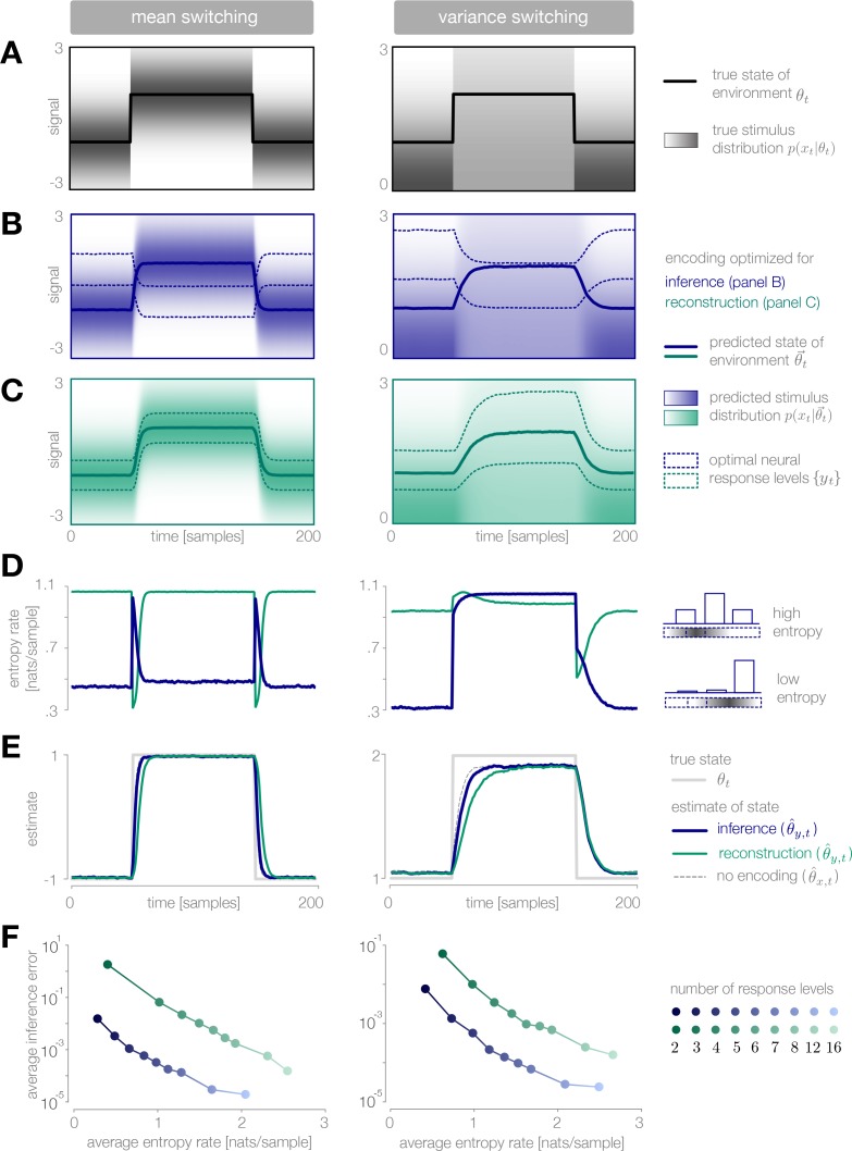
Figure 3. Dynamic inference with optimally-adapted response levels.

(A) We consider a probe environment in which a state ${\displaystyle {\theta }_t}$ (solid line) switches between two values at fixed time intervals. This state parametrizes the mean (left) or the variance (right) of a Gaussian stimulus distribution (heatmap). (B, C) Optimal response levels (dotted lines) are chosen to minimize error in inference (blue) or stimulus reconstruction (green) based on the predicted stimulus distribution ${\displaystyle p\left(x_t|{\overrightarrow{\theta }}_t\right)}$ (heatmap). Results are shown for three response levels. All probability distributions in panels A-C are scaled to the same range, ${\displaystyle \left[0,0.4\right]}$. (B) Response levels optimized for inference devote higher resolution (narrower levels) to stimuli that are surprising given the current prediction of the environment. (C) Response levels optimized for stimulus reconstruction devote higher resolution to stimuli that are likely. (D) The entropy rate of the encoding is found by partitioning the true stimulus distribution (heatmap in panel A) based on the optimal response levels (dotted lines in panels B-C). Abrupt changes in the environment induce large changes in entropy rate that are symmetric for mean estimation (left) but asymmetric for variance estimation (right). Apparent differences in the baseline entropy rate for low- versus high-mean states arise from numerical instabilities. (E) Encoding induces error in the estimate ${\displaystyle {\hat{\theta }}_t}$. Errors are larger if the encoding is optimized for stimulus reconstruction than for inference. The error induced by upward and downward switches is symmetric for mean estimation (left) but asymmetric for variance estimation (right). In the latter case, errors are larger when inferring upward switches in variance. (F) Increasing the number of response levels decreases the average inference error but increases the cost of encoding. Across all numbers of response levels, an encoding optimized for inference (blue) achieves lower error at lower cost than an encoding optimized for stimulus reconstruction (green). All results in panels A-C and E are averaged over 500 cycles of the probe environment. Results in panel D were computed using the average response levels shown in panels B-C. Results in panel F were determined by computing time-averages of the results in panels D-E.

Figure 3—figure supplement 1. Learning of optimal response levels with Lloyd’s algorithm.

Optimization of three response levels (quantization levels) for reconstruction (green) differs from optimization for inference (blue). Regardless of the error function (distortion measure), the algorithm converges to an optimum.

Figure 3—figure supplement 2. Deviations from optimal inference due to transmission noise.

(A) We simulated the noisy transmission of stimulus representations to downstream areas by injecting additive Gaussian noise into the response of a discretizing encoder. (B) The output response $y_t$ of the encoder is a discretized version of the incoming stimulus (upper row, gray). The observer receives a noisy version of the response (lower row, blue). (C) The estimate ${\displaystyle {\hat{\theta }}_t}$ is robust at low-noise levels, but degrades significantly for high noise levels. Results are averaged over 500 cycles of the probe environment.