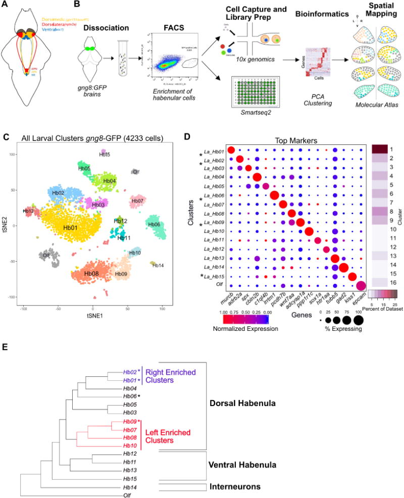
Figure 1. Unbiased Clustering of scRNA-seq Data Identifies 15 Molecular Distinct Neuronal Clusters in the Larval Habenula.

A. Schematic of the zebrafish habenula showing the anatomical subdivisions corresponding to the dorso-medial (orange), dorso-lateral (red) and ventral (blue) regions. These subdivisions are known to have distinct gene expression patterns and functionality.
B. Overview of the experimental strategy. Transgenic heads with gng8-GFP positive cells were dissected, pooled and dissociated, followed by enrichment of GFP+ habenular cells using fluorescent activated cell sorting (FACS). Single cell libraries were prepared using droplet-based droplet and plate-based Smart-seq2. Raw reads were processed to obtain a gene expression matrix (genes x cells). PCA and graph clustering was used to divide cells into clusters and identify cluster specific markers. Validation and spatial localization was performed using fluorescent RNA in situ hybridization (FISH) of statistically significant cluster-specific markers (see STAR Methods).
C. 2D visualization of single cell clusters using t-distributed Stochastic Neighbor Embedding (tSNE). Individual points correspond to single cells and are color-coded according to their cluster membership determined by graph-based clustering. The tSNE mapping was only used for post hoc visualization of the clustering but not to define the clusters themselves.
D. Gene Expression profiles (columns) of select cluster-specific markers identified through differential expression analysis (DEA) of previously known (labeled with an asterisk (*)) and new habenular types (rows). Bar on the right displays the percent of total dataset represented in every cluster, showing the abundance of each cell type found by clustering analysis.
E. A dendrogram representing global inter-cluster transcriptional relationships. The dendrogram was built by performing hierarchical clustering (correlation distance, average linkage) on the average gene-expression profiles for each cluster restricting to the highly variable genes in the dataset.
