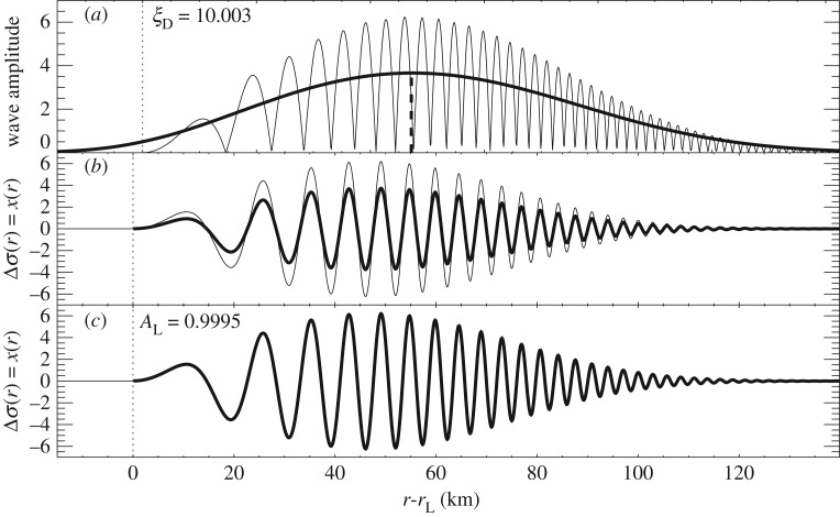
Figure 4.

(a) The absolute value of Δσ(r) (solid line); the same curve, smoothed three times with a 22 km boxcar filter, giving the low-frequency shape of the wave envelope (bold solid line); maximum point of the latter (vertical bold dashed line). (b) The input synthetic density wave from figure 2a (solid line); the fitted density wave, after the analysis of §4a(ii), but still with randomly chosen value of A_L (bold solid line). (c) The input synthetic density wave from figure 2a (solid line); the final fitted density wave, after the analysis of §4a(iii). Fitted values given in the figure can be compared with the input parameters (table 1) used to generate the wave. Figure from Tiscareno et al. [11].