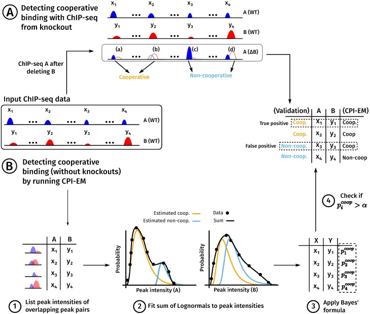
Fig 1. A schematic of the use of the CPI-EM algorithm and ChIP-seq from knockout data to separately identify cooperative bound transcription factor pairs.

ChIP-seq experiments carried out on two TFs, A and B, yield a list of locations that are bound by both TFs, along with peak intensities at each location. From this data, there are two ways in which we find genomic locations that are cooperatively bound by A and B. (A) A method for inferring these locations from a ChIP-seq of A carried out after B is genetically deleted. Locations where a peak of A either disappears altogether, or is reduced in intensity after knocking out B are labelled as cooperatively bound. In contrast, locations where a peak of A either remains unchanged or increases in intensity are labelled as non-cooperatively bound (see Materials and methods). (B) Steps in predicting cooperatively bound locations are shown, where the numbers correspond to those in the section “The ChIP-seq Peak Intensity—Expectation Maximisation (CPI-EM) algorithm” in Materials and Methods. (1) The input to CPI-EM consists of a list of genomic locations where a peak of A overlaps a peak of B by at least a single base pair. Note that the ChIP-seq of A after B is knocked out is not an input to the algorithm. (2) Each of these overlapping intensity pairs is fit to a model that consists of a sum of two probability functions. These functions specify the probabilities of observing a particular peak intensity pair given that it comes from a cooperatively or non-cooperatively bound region. These probabilities are computed by fitting the model to the input data using the expectation-maximization algorithm (see Section H in S1 Appendix). (3) Bayes’ formula is applied to the probabilities computed in step (2) to find the probability of each peak intensity pair being cooperatively bound. (4) Each cooperative binding probability computed in step (3) that is greater than a threshold α is declared as cooperatively bound. We compare this list of predicted locations with the list of cooperatively bound locations inferred from knockout data in order to compute the number of correct and incorrect inferences made by CPI-EM.