Laplace-based modeling of fiber orientation in the tongue

Abstract

Mechanical modeling of tongue deformation plays a significant role in the study of breathing, swallowing, and speech production. In the absence of internal joints, fiber orientations determine the direction of sarcomeric contraction and have great influence over real and simulated tissue motion. However, subject-specific experimental observations of fiber distribution are difficult to obtain; thus, models of fiber distribution are generally used in mechanical simulations. This paper describes modeling of fiber distribution using solutions of Laplace equations and compares the effectiveness of this approach against tractography from diffusion tensor magnetic resonance imaging. The experiments included qualitative comparison of streamlines from the fiber model against experimental tractography, as well as quantitative differences between biomechanical simulations focusing in the region near the genioglossus. The model showed good overall agreement in terms of fiber directionality and muscle positioning when compared to subject-specific imaging results and the literature. The angle between the fiber distribution model against tractography in the genioglossus and geniohyoid muscles averaged 22° likely due to experimental noise. However, kinematic responses were similar between simulations with modeled fibers versus experimentally obtained fibers; average discrepancy in surface displacement ranged from 1 to 7 mm, and average strain residual magnitude ranged from 4 × 10⁻³ to 0.2. The results suggest that, for simulation purposes, the modeled fibers can act as a reasonable approximation for the tongue’s fiber distribution. Also, given its agreement with the global tongue anatomy, the approach may be used in model-based reconstruction of displacement tracking and diffusion results.

1 Introduction

The human tongue is involved in multiple vital transport processes such as breathing, swallowing, and speech generation (Stone et al. 2016). These processes are elicited by tissue deformation arising from sarcomeric contraction (Gilbert et al. 2007). Sarcomeres are spatially arranged in fibers, which can curve and intersect in three-dimensional space (Takemoto 2001; Sanders and Mu 2013). The spatial distribution of fiber orientations is part of the tongue’s mechanical makeup through structure and constitutive behavior (Kajee et al. 2013; Harandi et al. 2017). The distribution is also involved in electrical propagation across the organ and wave excitation on its surface (Seiden and Curland 2015). Therefore, accurate fiber distribution modeling should be included in computational models to improve the agreement with experimental observations.

As there are no joints or rigid support structures within the tongue, other morphological adaptations are responsible for the organ’s ability to achieve the various shape configurations, which are required for its function (Gilbert et al. 2007). Thus, though myofibers also enable motion throughout the musculoskeletal system and in the heart (Anderson et al. 2007; Heemskerk and Damon 2007), the tongue is unique in that it contains interdigitation (intersection) along most of its volume and is capable of voluntary activation of independent muscle groups (Takemoto 2001; Stone et al. 2016).

The structure of the tongue has been studied though gross dissection, histological sections, and noninvasively, such as in diffusion tensor magnetic resonance imaging (DT-MRI) (Sanders and Mu 2013; Takemoto 2001; Gaige et al. 2007). The average adult tongue is roughly 90 mm long in the anteroposterior direction, and its width varies from roughly 30 mm near the tip to 60 mm in the middle, and 50 mm at its base (Sanders et al. 2013). Muscular bundles are layered, and laminae can be observed extending across the tongue’s volume, with smaller sections (such as the inferior longitudinalis (IL) muscle) being in the order of 10 mm by 5 mm, and larger structures encompassing roughly the entire tongue (Takemoto 2001). Transversally, laminae are roughly 200 μm wide with relatively wide gaps (200–300 μm) that allow intersection with layers arranged in orthogonal directions (as shown in Fig. 1) and exchange of interstitial fluids. Laminae are formed by tightly packed cells with diameters in the order of (40 μm), which elongate and arrange almost continuously along parallel directions (Saito and Itoh 2003; Mu and Sanders 2010). Tongue myofibers, then, cross at roughly right angles (Takemoto 2001), which enables independent motion in all three directions through conservation of volume (Gilbert et al. 2007). Although the general arrangement of fibers has been described in several studies, fiber orientation data, i.e., volumetric definitions of fiber directions, that can be included in computational models are not broadly available.

Fig. 1.

Arrangement of fibers and diffusion in the tongue. Tongue muscle fibers are layered in sheet-like laminae (a shown as a sagittal cross section). When sectioned perpendicularly, laminae follow a primary direction and, if interdigitation occurs, they have gaps that enable transverse intersection with another layer. Water diffusion in anisotropic media with one fiber family (b) results in clear differences between the primary (ev₁) and the remaining diffusion directions. When two fiber families are present (c), similar diffusivity rates can occur along two directions, resulting in directional ambiguity between the primary and the other principal diffusion directions. The tissue diagram was based on dissections. More details appear in Sanders et al. (2013), Saito and Itoh (2003), Mu and Sanders (2010)

The scarcity of model-ready fiber distribution data stem largely from difficulties associated with extraction of accurate numerical data from experimental observations. For instance, histological sections are precise, but only defined in a small cross sections, which are difficult to assemble into a 3D volume (Song et al. 2013). Likewise, quantification of fiber orientation from dissections, although demonstrated in the heart (LeGrice et al. 1995), has not yet been executed in the tongue, where observations have been broadly qualitative (Takemoto 2001; Mu and Sanders 2010). Measurements from DT-MRI generally consist of principal diffusion directions (an orthonormal basis) or fiber tracts, both of which can be directly imported into a model. In principle, the DT-MRI approach is advantageous because it provides noninvasive, subject-specific structural characterization (particularly in areas where a primary fiber direction dominates the diffusion tensor reconstruction) (Shinagawa et al. 2008; Gaige et al. 2007). However, despite its advantages, DT-MRI data can suffer from noise and spatial distortion (Gaige et al. 2007; Hageman et al. 2009). Further, as shown in Fig. 1, the presence of two or more fiber families, which is the case in interdigitated tongue muscles, can result in similar diffusivity along multiple directions—resulting in directional ambiguity with respect to the underlying structures, and lowering the confidence in directional measurements (Hageman et al. 2009). A realistic, simple, and repeatable model of fiber directionality can help with construction of simulations when experimental data are incomplete or nonexistent and can be used to better interpret experimental measurements.

Here, we investigate the use of Laplace-based, or rule-based, fiber modeling in the tongue. The method was originally designed to construct synthetic myofiber distributions in the heart (Bayer et al. 2012). The main premise consists of constructing a vector field (which represents fiber directions) from the spatial gradient of scalar potentials. These potentials arise from solving the Laplace equation in the same domain to be modeled according to strategically placed Dirichlet boundary conditions (Bayer et al. 2005). The vector field can then be manipulated by a set of rules to provide the final result. The goal of this study is to describe how this strategy can be used in the tongue and to assess the efficacy of the method with respect to the tongue anatomy, experimental observations from DT-MRI, and mechanical simulations.

2 Methods

2.1 Fiber modeling

We constructed a template finite-element (FE) mesh using a high-resolution atlas of the tongue and surrounding tissues (Woo et al. 2015). The FE model of the tongue, as illustrated in Fig. 2, was the geometric basis for fiber orientation modeling and was divided into volumetric muscular compartments containing unique combinations of muscles and fibers according to the literature (Stone et al. 2016; Sanders and Mu 2013; Takemoto 2001). Independent muscles could then be independently controlled in terms of activation, and the entire domain could be grouped into geometrical subdomains for fiber orientation generation. The model contains the intrinsic muscles including the superior longitudinalis (SL), inferior longitudinalis (IL), verticalis (V), and transversalis (T) and the largest extrinsic muscles including the genioglossus (GG), styloglossus (SG), and hyoglossus (HG), as well as the geniohyoid (GH).

Fig. 2.

Tongue model. This finite-element representation of the model was used to solve the Laplace equation for fiber generation and for mechanical simulations. The mesh a included several muscular compartments b and c including superior longitudinal (SL), inferior longutudinal (IL), verticalis (V), transversalis (T), genioglossus (GG), styloglossus (SG), hyoglossus (HG), and geniohyoid (GH). (Directional reference A anterior, P posterior, S superior, I inferior, L left, R right)

To obtain modeled fiber distributions, the Laplace equation was solved in subdomains of the finite element model (Bayer et al. 2005). The subdomains (in Fig. 3) were based on the muscular groups according to anatomical observations of myofiber aggregation. Boundary conditions were assigned to model the directional flow of myofibers using muscular origins as follows: to represent the general direction of the GG, a potential of zero was assigned at the origin behind the frontal apex of the mandible, while a potential of one was assigned along the dorsal surface. Longitudinal fibers for the SL and IL were modeled with boundary values of zero at the hyoid bone, and boundary values of one at the tip of the tongue. The transverse direction for the T was obtained by placing opposite boundary values on the left and the right. Potentials wrapping around the tongue were obtained by setting boundary values on either side to mimic the HG origin on either side. After setting boundary conditions, potential distributions, color maps in Fig. 3, were obtained using the thermal solver in the FEBio software suite (Maas et al. 2012), assuming each subdomain to be an isotropic medium with conductivity and diffusivity coefficients equal to 1. Solution time was less than 1s since only a single matrix, or one matrix inversion was necessary to achieve a solution.

Fig. 3.

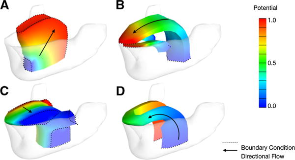
Laplace solutions. The color maps represent the scalar potential value within each of the subdomains, which include the GG superstructure (a), the longitudinal directions (b), the transverse directions (T), and inferior circumflex (d)

The vector field representing fiber orientations was obtained by calculating the spatial gradient of the scalar potentials defined at the nodes of the FE subdomains (Bayer et al. 2012). The gradient was calculated using isoparametric interpolation (Bathe 1996). This interpolation method establishes a mapping between the continuous spatial coordinates X and the local coordinates ξ through the discrete nodal coordinates X_a, by

$$X(\xi )={\displaystyle \sum _{a=1}^M{N}_a(\xi )X_a,}$$ (1)

where N_a (a = 1, 2, …, M) are the element’s shape functions according to the different element primitives used throughout the model (discussed in the Mechanical Modeling section below). Similarly, for a scalar function s defined at the nodes (s_a),

$$s(\xi )={\displaystyle \sum _{a=1}^M{N}_a(\xi )s_a.}$$ (2)

In this case, s_a is the potential obtained after solving the Laplace equation. The spatial gradient of the potential, and subsequent fiber orientation model,

$$\nabla s(\xi )={\displaystyle \sum _{a=1}^M{s}_a\frac{\partial N_a(\xi )}{\partial X}}$$ (3)

was obtained via

$$\nabla s(\xi )={\displaystyle \sum _{a=1}^M{s}_a{\frac{\partial X}{\partial \xi }}^{-T}\frac{\partial N_a}{\partial \xi },}$$ (4)

which involves calculating the derivatives of the shape functions with respect to the local coordinates (i.e., $\frac{\partial N_a}{\partial \xi }$), and

$$\frac{\partial X}{\partial \xi }={\displaystyle \sum _{a=1}^M{X}_a\otimes \frac{\partial N_a}{\partial \xi }},$$ (5)

where ⊗ denotes the matrix outer product. The calculations associated with (4) were performed using a custom script in MATLAB (Natick, MA, USA). Note that the isoparametric formulation is convenient because each integration point can be expressed in terms of local coordinates where, for instance, ξ = [0 0 0]^T represents the centroid. If nodal values are required instead of centroidal values, gradients can be evaluated at the nodes and averaged across the elements that share the node.

The final fiber orientation vector field was found by consolidating the gradients according to the muscles in each muscular compartment. Most of the muscles simply inherit the gradients calculated from the subdomains in Fig. 3. (For instance, Laplace-based fibers evaluated at element centroids in the muscular compartments in Fig. 2c is shown in Fig 4a.) However, fiber directions for the V are obtained by imposing a rule in the compartments associated with this muscle, where the fibers arise from the cross product of the longitudinal and transverse directions. Because some muscles are interdigitated, two fiber families were defined based on two superimposed potential distributions in the same muscular compartment. For example, compartment 3 in Fig. 2b contains fibers from the potential gradient in Fig. 3b, (for the SL), as well as the cross product between the gradients of the potentials in Fig. 3c and d (for the V).

Fig. 4.

Fiber distribution sources. Laplace-based fibers a were defined from the spatial gradient of scalar potential. Tractography-based fibers b were obtained from experimental imaging results using DT-MRI

2.2 Experimental observations

Experimental observations of fiber distributions were obtained using DT-MRI of healthy volunteers. One scan with high-directional resolution (200 diffusion-encoding directions) was acquired for qualitative comparison, while additional standard resolution scans (n = 4, 2 males, 2 females) were used to derive fiber orientations for subject-specific biomechanical modeling.

DT-MRI was performed using a Siemens Prisma Fit 3.0 T scanner (Siemens Healthcare, Erlangen, Germany). Single-shot 2D spin-echo echo planar imaging (EPI) was applied with the following parameters: TR = 2.5 s with no TR delay, TE = 57 ms, field of view 240 mm, 30 slices, 3 mm slice thickness, matrix size 80 80 with an image pixel size 3 mm × 3 mm, bandwidth× 2500 Hz/px, b = value 500 s/mm², 5 non-diffusion weighted volumes, 63 (standard) or 200 (high-resolution) diffusion gradient directions, with multislice mode interleaved.

Tractography was used as an experimental measurement to compare the fiber modeling results. Tracts were used to reconstruct fiber distributions in the subjects and as an alternative means to extract fibers for biomechanical models. The tractography results were obtained using Trackvis (track-vis.org) and DSI studio software (dsi-studio.labsolver.org), assuming that diffusion can be modeled by a single tensor to extract local fiber directions. (Reliable multi-fiber reconstruction for the tongue is not yet available.) Fiber orientation was reconstructed from the tracts by calculating the local tangent at each tract node and transferring it to the closest evaluation point in the mesh. Unlike other modeling approaches that use diffusion eigenvalues directly (Vadakkumpadan et al. 2010), we used tractography to reduce directional ambiguity and to smooth data, because tracts include directionally constraints along the path and spline smoothing is built into the tractography algorithms. This approach also simplifies vectorial interpolation. A sagittal view of the tract-based fibers used in the muscular compartments in Fig. 2c is shown in Fig 4b. The overall approach for comparing fiber modeling and experimental observations is shown in Fig. 5.

Fig. 5.

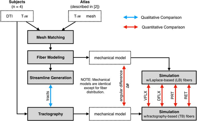
Comparative experiments. Subject-specific models were generated by matching a template mesh (in Atlas space) to anatomical images of each subject (n = 4). Qualitatively, pseudo-fiber distributions from Laplace-based streamlines were compared against tractography. Quan titatively, fiber directions were compared directly in the mesh, and by measuring differences in 4 simulated deformations shown in Fig. 6. (T₁w denotes T₁-weighted images.)

2.3 Biomechanical model

The FE mesh used for fiber modeling was also used to generate simulated motion using contraction as one of the inputs (forward modeling). The FE mesh comprised 300 tetrahedral elements (for the bones), 255 quadratic hexahedral elements with 20 nodes points each (for the tongue), and 24 spring elements (for the SG). The geometry and location of the mandibular bone, hyoid bone, and the SG were obtained from manual delineations of the atlas. Note that quadratic elements were used so that the space between evaluation points for fiber orientation was lower than the DT-MRI resolution. Element definition within the tongue followed a structure described in the published literature (Fujita et al. 2007). Constitutively, the bones were assumed to be rigid, and the passive material response of the tongue was modeled using an uncoupled formulation of a fourth-order, nearly incompressible, Mooney–Rivlin solid. Based on previous computational studies (Harandi et al. 2015; Stavness et al. 2012), the coefficients were adjusted to match static elastic moduli with C₁₀ = 1040 kPa, C₂₀ = 490 kPa, and C₀₁ = C₀₂ = 0. The bulk modulus was 100 kPa, and the spring elements were assigned a Young’s modulus of 12 (nearly rigid).

Mechanical loading was achieved through simulated contraction using FEBio (Maas et al. 2012). To this end, the material response in the tongue was modeled as a solid mixture of the passive response described above and a Hill formulation of active sarcomeric length- dependent stress, assuming a maximum stress of 135 kPa (Guccione et al. 1993; Guccione and McCulloch 1993). (More details on the implementation of active contraction appear in the “Appendix”.) The mechanical boundary conditions consisted of rigid contacts between the tongue and the mandibular bone at the origin of the GG, and between the hyoid bone and the origins of the HG and SL. The mandible was allowed to rotate freely about the left-to-right axis anchored at the approximate location of the styloid process. The hyoid bone was allowed to rotate freely about the same axis of rotation as the mandible, except that the anchor point was located near the closest contact with the trachea. The remaining degrees of freedom were constrained for simplicity although, in reality, the hyoid bone is free to displace and rotate in additional ways.

Subject-specific models were constructed by matching the template model to the anatomy of each of the four volunteers (Fig. 5). Matching was performed by manual affine registration using anatomical landmarks including the mandibular and hyoid bones, as well as the location of the hard palate, styloid process, the tip of the tongue, and the base of the GG muscle. The mean distance between integration points in the atlas was 2.66 ± 1.1 mm, and in the subject-specific models ranged from 2.00 ± 0.9 to 2.34 ± 1.0 mm, which is similar to the DT-MRI resolution (3 mm). Overall similarity between mesh size among volunteers dismissed the need for mesh refinement based on size differences. The subject-specific mechanical models were labeled S1 through S4 and used for simulations as described in Sect. 2.4 below.

2.4 Experiments

The experimental approach is illustrated in Fig. 5.

2.4.1 Qualitative comparison

The goal of this experiment was to assess the overall agreement between the Laplace-based fiber distributions and those obtained with actual acquired. To visualize the modeled fibers, streamlines were generated from the potential gradients evaluated at the mesh nodes using the streamline generation algorithm in the Visit visualization software (Lawrence Livermore National Laboratory, Livermore, CA, USA). The result was compared against tractography results from high-resolution DT-MRI focusing on areas governed by one diffusivity direction (see Fig. 5).

2.4.2 Differences between simulations with experimental and modeled fiber orientation

The goal of this experiment was to quantify changes in simulated motion when modeled fiber distributions are used as a substitute for experimentally obtained fiber directions. The extent of the comparison was reduced to compensate for limitations in the experimental measurements from DT-MRI, which prevent comparison across the entire tongue. Instead, we focused on the GG and GH muscles (i.e., the muscular compartments shown in Fig. 2c). The GG is the largest muscle in the tongue and has the most varied fiber direction (Gilbert et al. 2007; Stone et al. 2016). The GH is a muscle in the floor of the mouth that originates and inserts on bone unlike the other muscles of the tongue, with fibers along a single, dominant direction, which provides contrast with the GG. These regions also lend themselves to diffusion-based measurements, which have the greatest agreement with direct observation of fiber distribution using other techniques in the same region (Gilbert et al. 2007; Aoyagi et al. 2015; Takemoto 2001).

Two versions of each subject-specific mechanical model were constructed: one with Laplace-based (LB) fibers and one including tractography-based (TB) fibers. In the LB mechanical model, fiber directions were assigned by evaluating (4) at each integration point, as described in Sect. 2.1. In the TB model, fibers were assigned as follows: The primary direction in muscular compartments associated with the GG and GH (Fig. 2c) were obtained purely from tractography; the secondary direction in these compartments (affecting the T and SL) was obtained by performing the cross product of the primary direction from tractography and (4), which was used in the secondary direction; the remaining compartments were derived solely from (4).

Simulated states of contraction were obtained by modulating the active stress as a percentage of the maximum (135 kPa as described in the Mechanical Modeling section). The simulations focused on different muscular compartments according to whether the fibers were LB or TB, and not necessarily on the representation of physiological cases. However, we focused on a limited basis of motion for speech generation in healthy humans that did not include asymmetric (left-to-righ) movement. The simulations consisted of ventroflexion (VFLX), which lowers the tip of the tongue; dorsiflexion (DFLX), which elevates the tip of the tongue; protrusion (PRT), which moves the tongue forward; and retraction (RET), which moves the tongue backward. Active stress is distributed according to Table 1, and the simulated deformed states are shown in Fig. 6. The activation profiles were obtained by trial and error after inspecting the simulated results with the help of the literature (Sanguineti et al. 1997; Perrier et al. 2003).

Table 1.

Active stress distributions. This input to the mechanical simulations determines the simulated deformation

Muscle	VFLX %	DFLX %	PRT %	RET %
GG	50.0	0.0	7.0	0.0
GH	0.0	0.0	7.0	0.0
HG	0.0	0.0	0.0	35.0
IL	0.0	0.0	0.0	28.0
SG	0.0	0.0	0.0	70.0
SL	0.0	50.0	15.0	2.0
T	0.0	0.0	33.0	0.0
V	0.0	0.0	33.0	0.0

SL superior longitudinal, IL inferior longutudinal, V verticalis, T transversalis, GG genioglossus, SG styloglossus, HG hyoglossus, GH geniohyoid

Fig. 6.

Simulations in their deformed configuration. The outline of the reference configuration (dotted line) shows the undeformed state. The simulations included ventroflexion, or VFLX (a), dorsiflexion, or DFLX (b), protrusion, or PRT (c), and retraction, or RET (d). (Directional reference A anterior, P posterior, S superior, I inferior, L left, R right)

Two quantities were used to compare LB against TB models: magnitude of motion in the dorsal surface in each model and strain residuals. The first metric was chosen because the tongue’s surface has a significant overall contribution to speech generation and breathing (Harandi et al. 2017). It is defined as

$${\epsilon }_s=\Vert {\mathit{x}}_{\text{LB}}-{\mathit{x}}_{\text{TB}}\Vert ,$$ (6)

where x_LF and x_TF represent the coordinates of nodes along the dorsal surface in the deformed configuration for the LB and TB models, respectively. (We use ║ to denote the matrix 1–2 norm.) When simulations are identical, ε_s = 0 mm. The second metric quantifies the differences in deformation profiles

$${\epsilon }_E=\Vert {\mathit{E}}_{\text{LB}}-{\mathit{E}}_{\text{TB}}\Vert ,$$ (7)

where E represents the Green–Lagrange strain tensor (Spencer 1985). If ε_E = 0, the two simulations being compared are identical. In terms of physical interpretation, ε_E is a conservative measure of strain error if it is assumed that ε_E > 0 arises from a single diagonal component of E, because most of the time error will be distributed on 6 unique components. Both metrics were averaged in each pair of models across all nodes (for ε_s) or elements (for ε_E). Surface error ε_s was projected to the deformed surfaces for visualization.

To aid with the interpretation of results, error quantifications per (6) and (7) were plotted against the mean angle between modeled and experimental fibers Δθ (see Fig. 5). Additional simulations were performed using the template mesh to estimate the sensitivity of error metrics to changes in fiber direction. To this end, a pair of simulations was created for each activation profile. The first simulation of the pair used Laplace-based fibers. In the other, the Laplace-based fibers were rotated at random using a normal distribution with a mean and a standard deviation of 0°, 10°, 20°, 30, and 40°. Comparing each pair allowed calculation of Δθ, ε_s, and ε_E as a reference for the other results.

3 Results

3.1 Tractography

Streamlines obtained from the modeled fiber distribution are shown in Fig. 7. The GG muscle exhibits a fan-like pattern, which is observed in the modeled streamlines (Fig. 7a) and experimental tracts (Fig. 7b). Likewise, the GH shows fibers along the anteroposterior direction, which is also the case in both sets of tracts. Unlike the modeled fibers, the experimental tracts exhibit a separation between the GG and the HG. As with the GG and GH, the IL, and SG flow in similar directions (note that the projected view of the experimental fibers from the right side also shows some SG fibers belonging to the left side, which seem to appear in the posterior of the tongue). In general, the modeled fiber distribution resulted in well-defined longitudinal, transverse, and vertical trajectories that are relatively consistent across the tongue volume. In contrast, experimental results show more directional variation along the tracts and larger areas of what appear to be incomplete results. For instance, the directions of the V and the T appear more inconsistent in the experimental results than in the model, and tracts along the SL stop before bending inferiorly in the posterior of dorsal surface. As expected, experimental tractography was unable to resolve transverse fibers crossing the GG and the V, likely due to the single dominant direction assumption from single tensor reconstruction.

Fig. 7.

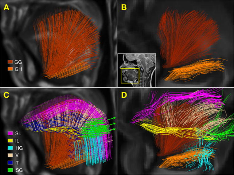
Comparison between modeled and experimentally obtained tracts. The modeled GG and GH tracts a have approximately the same color as the experimental b tractography results. The arrows in the whole tongue view of the modeled tracts c represent the direction of SG spring elements. No transverse fibers appear in the whole tongue view of the experimental tractography d likely due to the single fiber assumption

3.2 Differences between simulations with experimental and modeled fiber orientation

3.2.1 Qualitative comparison

Dorsal surface maps in the deformed configuration of each simulation are shown in Fig. 8. The shape of each surface was determined by the simulation with TP fiber distribution. In the best case scenarios, error measured via ε_s was less than one-tenth of a millimeter. The largest overall ε_s was 6.6 mm in the VFLX simulation corresponding to Subject 4 (S4). In the best-performing simulation, RET (S2), the largest error value was 0.2 mm. Fiber distribution changes were more apparent in some simulations than others. For instance, the top row (VFLX) had larger overall values of ε_s than the middle rows (DFLX and PRT). The bottom row (RET) exhibited the smallest error values. While the distribution of ε_s shows that error occurred throughout the dorsal surface, some error concentrations appear to affect the tip of the tongue. The small overall error across all models and simulations is evidence that the TB deformed configurations were similar to their LB counterparts (notwithstanding the differences in shape between the models): as expected from Fig. 6, simulations of VLFX tended to extend the dorsal surface as the tip lowers; DFLX simulation resulted in a shortened dorsal surface with an elevated tip; similarly, simulation of PRT and RET resulted in relative motion of the tip along the anterior or posterior directions, respectively.

Fig. 8.

Dorsal surface position error maps. Error between simulations with Laplace-based (LB) and tractography-based (TB) fiber distribution ε_s was projected on the deformed configuration of subject-specific simulations S1 through S4. The number represents the spatial mean ε_s with the standard deviation in parenthesis. (VFLX ventroflexion, DFLX dorsiflexion, PRT protrusion, RET retraction.)

Mean strain error, or ε_E, is shown in Table 2. The general pattern of error across subjects and simulations is similar to ε_s; the largest values appeared in VLFX simulations, and the smallest in RET simulations. The average angle between LB and TB fiber directions was largest in S4 at 28° ± 13, and smallest in S2 at 17° ± 15. (The same measurements were 23° ± 20 and 22° ± 17 in S1 and S3, respectively).

Table 2.

Magnitude of the strain residual between simulations with Laplace-based and tractography-based fiber distribution ε_E. Subject-specific simulations are labeled S1 through S4. Numerical values represent the spatial mean with the standard deviation in parenthesis. (Strain is a dimensionless quantity.)

	S1	S2	S3	S4
VFLX	0.158 (0.106)	0.136 (0.068)	0.148 (0.080)	0.206 (0.073)
DFLX	0.070 (0.046)	0.071 (0.055)	0.058 (0.033)	0.075 (0.058)
PRT	0.075 (0.040)	0.063 (0.037)	0.072 (0.036)	0.101 (0.044)
RET	0.005 (0.004)	0.005 (0.005)	0.004 (0.004)	0.006 (0.006)

Plots of ε_s and ε_E against the mean angle between modeled and experimental fibers Δθ are shown in Fig. 9. Generally speaking, disagreement in simulated outcomes (per ε_s and ε_E) increases as a function of the angle between two fiber distributions, that is, the model outcomes are sensitive to fiber orientation. However, the amount of change that can be expected with a given directional variation, i.e., the rate of change of error to changes in fiber orientation, varies drastically depending on the activation profile. Figure 9 shows that the simulations can be ordered according to their sensitivity, starting with the most sensitive, as: VFLX, PRT, DFLX, and RET. Both the amount of error and the rate of error increase as a function of Δθ; for example, at Δθ = 40° in VFLX, ε_s is roughly 9 mm (a 2-fold change from Δθ = 30°). The subject-specific simulations show similar trends of error sensitivity and error rates.

Fig. 9.

Error as a function of directional variability. In the subject-specific models (outlined circles), Δθ represents the angle between Laplace-based and tractography-based fiber directions. In the sensitivity results (dotted lines), error represents the difference between a reference simulation and a simulation where fibers were deliberately rotated at random; thus, Δθ represents the mean and standard deviation of a normal distribution. (−) denotes dimensionless units. (Simulations VFLX ventroflexion, DFLX dorsiflexion, PRT protrusion, RET retraction.)

4 Discussion

Fiber arrangement in the tongue has previously been described in terms of a fan-like core (mostly the GG) surrounded by inferior and superior longitudinal arrangement (the IL and SL muscles) and an arrangement of transverse fibers in the left-to-right direction (Sanders and Mu 2013; Takemoto 2001). By design, our modeling strategy incorporates these observations as shown in Fig 6. The main feature in the model is a fan-like superstructure containing the GG and GH originating at the inner anterior surface of the mandible. The directional distribution in the model also reflects previous work describing strong interdigitation between the GG, T, and V in the middle of the tongue as shown in Fig. 7c (Takemoto 2001). Likewise, the modeling strategy gives rise to an SL flowing posteriorly from the tip of the tongue bending in the inferior direction and almost merging (per its direction) with the HG toward the posterior base the tongue on the superior side of the hyoid bone. The IL starts near the tip of the tongue and flows posteriorly starting with a concave curvature (concave down), which becomes more convex posteriorly (Stone et al. 2016). The SG fibers are located on the tongue’s sides pointing superiorly toward the styloid process. The LB fiber orientation models features that agree with prior experimental observations, demonstrating its potential for both modeling purposes and for detection (and measurement) of deviation from the expected arrangement of fibers due to disease or experimental error.

The DT-MRI results show key similarities to the LB fiber distribution, but there are also some differences. The most notable agreement was observed in the GG and GH, with the IL also showing some overall agreement. Similar directionality could also be appreciated in the SL, and V, but the agreement was partial. (For instance, the SL does not curve posteriorly in the experimental data.) The HG and SG exhibited the least visual agreement, as these muscles have a thickness similar to the imaging resolution (about 3 mm), which makes them susceptible to partial volume effects. (The same is also true near the IL and thin parts of the SL.) DT-MRI did not produce transverse fibers within the GG as most fibers aligned in the local GG direction. The DT-MRI results also exhibit gaps and changes in directions (or waviness) at a scale that would not be expected assuming some smoothness of muscle tissue. These experimental flaws are most likely a product of reconstruction of diffusion data, which has to maintain a balance between directional sensitivity for generating tracts in coherent directions, and robustness to noise to avoid excessive waviness (Hageman et al. 2009). The presented single tensor reconstruction has the advantage of being fairly robust to noise enabling acquisition in vivo. However, this method also results in directional ambiguity in areas with crossing fibers, which are the most likely cause of apparent gaps, the lack of curvature of the SL, and the absence of transverse tracts, which can also be seen on other studies (Gaige et al. 2007). These shortcomings could be mitigated in future studies by coupling multi-tensor reconstruction with motion-tolerant acquisition techniques. Despite these experimental flaws, the imaging results show substantial consistency with the model, as the areas with the most agreement (GG, GH, IL and part of the SL) include some of the largest functional volumes in the tongue (Stone et al. 2016).

While some directional disagreement between simulated and experimentally derived fibers was measured (per Δθ), the results in Figs. 8, 9, and Table 2 show that simulations with LB fibers are equivalent to the simulations obtained with experimentally derived TB fibers within reasonable accuracy. One difficulty interpreting the measurements of Δθ alone is in establishing the quality of the diffusion-based reconstructions as a ground truth. On one hand, DT-MRI measurements, including those in this study and the literature (Gilbert et al. 2007; Shinagawa et al. 2008), have been shown to correlate well with the macroscopic arrangement of tongue muscles, which is the target of this investigation. On the other hand, these measurements show some level of directional heterogeneity as seen in Figs. 4 and 7d, particularly bearing in mind that tractography is a smooth representation of the DT-MRI results, which would have increased the variability of Δθ if defined between LP fibers and the primary diffusion direction. Given the macroscopic agreement between the fiber model and the experimental observations, it is more likely that the local differences measured via Δθ reflect experimental variability and not global disagreement. In contrast, analysis using the metric ε_s shows relatively low average values in a maximum dorsal surface position error. As an average across subjects, this error is in the order of 2 mm (Fig. 9), which is similar to the average tracking accuracy of experimental tongue motion (Harandi et al. 2017) and is unlikely to have profound impact in speech-related simulations. In terms of strain, the largest tensor magnitude ε_E was roughly 0.2 (Table 2), averaging 3% across the 6 free parameters of strain, depending on the local deformation. These values were extracted from VFLX, which given its sensitivity to Δθ is the most conservative assessment of performance of those studied. As Fig. 9 shows, the VFLX simulation can result in larger error values, but this did not occur given that Δθ did not exceed 28°. Note that Δθ could be further improved by improving registration from the atlas template to the subjects. Mesh matching has been successfully employed to reproduce dynamic tongue data in subject-specific models in similar meshes (Harandi et al. 2017). Alternatively, Δθ can be improved by optimizing the boundary conditions in the Laplace-generated fibers for each model, but these were held constant across all models to determine the effectiveness of using modeled fibers to replace experimental observations in cases where data is not available.

Although this study is comprehensive in the sense that it provides experimental and simulated data, it is limited in that comparisons were not performed across the entire tongue (due to limitations on the experimental measurements). Thus, the difference between simulations with LB and TB fibers was the largest in the GG–GH region (Fig. 2c). Therefore, simulations yielding stress distributions with relative large magnitudes within this region (as is the case in VFLX simulations) resulted in larger discrepancies than those where stress was concentrated elsewhere (e.g., RET simulations). Because the passive constitutive model was isotropic, differences between models as quantified by ε_E and ε_s were directly linked to active stress, giving rise to the sensitivity trends shown in Figs. 8 and 9. In VFLX, evaluation of active stress depended entirely on contraction within the GG, which contains the largest amount of fibers from the different sources being compared. Since VFLX the most sensitive simulation to changes in fiber orientation, it yielded in the largest errors, as seen in Fig. 8. Conversely, virtually all stress in the RET simulations was introduced at integration points outside the GG–GH region, which contributed only its passive isotropic response, yielding identical results despite differences in fiber distribution.

Given that the isotropic assumption is relatively common in tongue modeling, future research can focus on improved material characterization and reconstruction of fibers in 3D across the whole tongue. As a step forward, the presented methodology can be used to generate prior information to facilitate reconstruction of DT-MRI (Ye et al. 2016). Such an approach would leverage the agreement between the modeled fiber distribution and overall anatomical fiber orientations to guide the reconstruction process in areas of low signal or directional ambiguity. Further integration between the model and experimental data could mean that a model-based approach could also be used to identify disease or contractile deficiencies arising from interventions. Finally, future research is necessary to elucidate how fiber orientation affects the tongue’s electrophysiology, particularly as it may apply for more advanced electromechanical models.

5 Conclusion

We described an approach to model fiber distribution in the tongue using solutions to the Laplace equation. This methodology is relatively simple to implement in existing geometry, and the results agree with anatomical descriptions. The resulting fiber distributions also demonstrate functional equivalence with respect to results from DT-MRI when used in simulations using subject-specific models. The proposed method can be applied in biomechanics simulations, as shown here, and may also be useful in diffusion MRI reconstruction and in the detection of kinetic abnormalities.

6 Appendix

6.1 Additional details on active contraction

In order to simulate the sarcomeric contraction that gives rise to tongue motion, the simulated Cauchy stress tensor T was calculated as the sum of a passive and an active contribution. The active component T_act was defined with respect to maximum isomeric stress T_max at peak calcium concentration ${({\text{Ca}}_0^2)}_{max}=4.35\mathrm{\mu }\mathrm{M}$. More specifically,

$${\mathit{T}}_{\text{act}}=T_{max}\frac{{\text{Ca}}_0^2}{{\text{Ca}}_0^2+{\text{Ca}}_{50}^2(l)}C(t),$$ (8)

where C(t) is an increasing load curve for the iterative solver, which is scaled according to the required level of activation, e.g., the values in Table 1 (Guccione et al. 1993). The phenomenological relationship

$${\text{ECa}}_{50}^2(l)=\frac{{\text{Ca}}_0^2}{\sqrt{e^{B(l-l_0)}-1}}$$ (9)

describes calcium sensitivity, which depends on intracellular calcium concentration ( ${\text{Ca}}_0^2$), and sarcomere length l. This dependency is important because, as in reality, no more stress will be developed once sarcomeres retract in full. Experimentally, B = 4.75μm⁻¹, and the length at which sarcomere tension stabilizes l₀ = 1.58μm. The current length l is found using the deformation gradient (Guccione et al. 1993; Guccione and McCulloch 1993).

References

- Anderson RH, Sanchez-Quintana D, Redmann K, Lunkenheimer PP. How are the myocytes aggregated so as to make up the ventricular mass? Semin Thoracic Cardiovasc Surg. 2007 doi: 10.1053/j.pcsu.2007.01.016. [DOI] [PubMed]
- Anneriet MH, Damon Bruce M. Diffusion tensor MRI assessment of skeletal muscle architecture. Curr Med Imaging Rev. 2007;3(3):152–60. doi: 10.2174/157340507781386988. [DOI] [PMC free article] [PubMed] [Google Scholar]
- Aoyagi H, Si I, Asami T. Three dimensional architecture of the tongue muscles by micro CT with a focus on the longitudinal muscle. Surg Sci. 2015 May;6:187–197. [Google Scholar]
- Bathe KJ. Finite element procedures. 2nd. Prentice-Hall; Upper Saddle River: 1996. [Google Scholar]
- Bayer JD, Beaumont J, Krol A. Laplace–Dirichlet energy field specification for deformable models. An FEM approach to active contour fitting. Ann Biomed Eng. 2005;33(9):1175–1186. doi: 10.1007/s10439-005-5624-z. [DOI] [PubMed] [Google Scholar]
- Bayer JD, Blake RC, Plank G, Trayanova NA. A novel rule-based algorithm for assigning myocardial fiber orientation to computational heart models. Ann Biomed Eng. 2012;40(10):2243–2254. doi: 10.1007/s10439-012-0593-5. [DOI] [PMC free article] [PubMed] [Google Scholar]
- Fujita S, Dang J, Suzuki N, Honda K. A computational tongue model and its clinical application. Oral Sci Int. 2007;4(2):97–109. doi: 10.1016/S1348-8643(07)80004-8. [DOI] [Google Scholar]
- Gaige TA, Benner T, Wang R, Wedeen VJ, Gilbert RJ. Three dimensional myoarchitecture of the human tongue determined in vivo by diffusion tensor imaging with tractography. J Magn Reson Imaging. 2007;26(3):654–661. doi: 10.1002/jmri.21022. [DOI] [PubMed] [Google Scholar]
- Gilbert RJ, Napadow VJ, Gaige TA, Wedeen VJ. Anatomical basis of lingual hydrostatic deformation. J Exp Biol. 2007;210(Pt 23):4069–4082. doi: 10.1242/jeb.007096. [DOI] [PubMed] [Google Scholar]
- Guccione JM, McCulloch AD. Mechanics of active contraction in cardiac muscle: part I—constitutive relations for fiber stress that describe deactivation. J Biomech Eng. 1993;115(1):72–81. doi: 10.1115/1.2895473. [DOI] [PubMed] [Google Scholar]
- Guccione JM, Waldman LK, McCulloch AD. Mechanics of active contraction in cardiac muscle: part II—cylindrical models of the systolic left ventricle. J Biomech Eng. 1993;115(1):82–90. doi: 10.1115/1.2895474. [DOI] [PubMed] [Google Scholar]
- Hageman NS, Toga AW, Narr KL, Shattuck DW. A diffusion tensor imaging tractography algorithm based on Navier–Stokes fluid mechanics. IEEE Trans Med Imaging. 2009;28(3):348–360. doi: 10.1109/TMI.2008.2004403. [DOI] [PMC free article] [PubMed] [Google Scholar]
- Harandi NM, Woo J, Farazi MR, Stavness L, Stone M, Fels S, Abugharbieh R. Subject-specific biomechanical modelling of the oropharynx with application to speech production. IEEE ISBI; 2015. [DOI] [Google Scholar]
- Harandi NM, Stavness I, Woo J, Stone M, Abugharbieh R, Fels S. Subject-specific biomechanical modelling of the oropharynx: towards speech production. Comput Methods Biomech Biomed Eng Imaging Vis. 2017;5(6):416–426. doi: 10.1080/21681163.2015.1033756. [DOI] [PMC free article] [PubMed] [Google Scholar]
- Kajee Y, Pelteret JPV, Reddy BD. The biomechanics of the human tongue. Int J Numer Methods Biomed Eng. 2013;29(4):492–514. doi: 10.1002/cnm.2531. [DOI] [PubMed] [Google Scholar]
- LeGrice IJ, Smaill BH, Chai LZ, Edgar SG, Gavin JB, Hunter PJ. Laminar structure of the heart: ventricular myocyte arrangement and connective tissue architecture in the dog. Am J Physiol Heart Circu Physiol. 1995;269(2):H571–H582. doi: 10.1152/ajpheart.1995.269.2.H571. [DOI] [PubMed] [Google Scholar]
- Maas SA, Ellis BJ, Ateshian GA, Weiss JA. FEBio: finite elements for biomechanics. J Biomech Eng. 2012;134(1):5-1–5-10. doi: 10.1115/1.4005694. [DOI] [PMC free article] [PubMed] [Google Scholar]
- Mu L, Sanders I. Human tongue neuroanatomy: nerve supply and motor endplates. Clin Anat. 2010;23(7):777–791. doi: 10.1002/ca.21011. NIHMS150003. [DOI] [PMC free article] [PubMed] [Google Scholar]
- Perrier P, Payan Y, Zandipour M, Perkell J. Influences of tongue biomechanics on speech movements during the production of velar stop consonants: a modeling study. J Acoust Soc Am. 2003;114(3):1582–1599. doi: 10.1121/1.1587737. [DOI] [PubMed] [Google Scholar]
- Saito H, Itoh I. Three-dimensional architecture of the intrinsic tongue muscles, particularly the longitudinal muscle, by the chemical-maceration method. Anat Sci Int. 2003;78(3):168–176. doi: 10.1046/j.0022-7722.2003.00052.x. [DOI] [PubMed] [Google Scholar]
- Sanders I, Mu L. A three-dimensional atlas of human tongue muscles. Anat Rec. 2013;296(7):1102–1114. doi: 10.1002/ar.22711. NIHMS150003. [DOI] [PMC free article] [PubMed] [Google Scholar]
- Sanders I, Mu L, Amirali A, Su H, Sobotka S. The human tongue slows down to speak: muscle fibers of the human tongue. Anat Rec. 2013;296(10):1615–1627. doi: 10.1002/ar.22755. NIHMS150003. [DOI] [PMC free article] [PubMed] [Google Scholar]
- Sanguineti V, Laboissière R, Payan Y. A control model of human tongue movements in speech. Biol Cybern. 1997;77(1):11–22. doi: 10.1007/s004220050362. [DOI] [PubMed] [Google Scholar]
- Seiden G, Curland S. The tongue as an excitable medium. New J Phys. 2015;17:1–7. doi: 10.1088/1367-2630/17/3/0330491402.2272. [DOI] [Google Scholar]
- Shinagawa H, Murano EZ, Zhuo J, Landman B, Gullapalli RP, Prince JL, Stone M. Tongue muscle fiber tracking during rest and tongue protrusion with oral appliances: a preliminary study with diffusion tensor imaging. Acoust Sci Technol. 2008;29(4):291–294. doi: 10.1250/ast.29.291. [DOI] [Google Scholar]
- Song Y, Treanor D, Bulpitt A, Magee D. 3D reconstruction of multiple stained histology images. J Pathol Inform. 2013;4(2):7. doi: 10.4103/2153-3539.109864. [DOI] [PMC free article] [PubMed] [Google Scholar]
- Spencer AJM. Continuum mechanics. 1995th. Dover Books; Essex: 1985. http://www.barnesandnoble.com/w/continuum-mechanics-anthony-james-spencer/1101818174?ean=9780486139470. [Google Scholar]
- Stavness I, Lloyd JE, Fels S. Automatic prediction of tongue muscle activations using a finite element model. J Biomech. 2012;45(16):2841–2848. doi: 10.1016/j.jbiomech.2012.08.031. [DOI] [PubMed] [Google Scholar]
- Stone M, Woo J, Lee J, Poole T, Seagraves A, Chung M, Kim E, Murano EZ, Prince JL, Blemker SS. Structure and variability in human tongue muscle anatomy. Comput Methods Biomech Biomed Eng Imaging Vis. 2016;1163:1–9. doi: 10.1080/21681163.2016.1162752. [DOI] [PMC free article] [PubMed] [Google Scholar]
- Takemoto H. Morphological analyses of the human tongue musculature for three-dimensional modeling. J Speech Lang Hear Res. 2001;44(1):95–107. doi: 10.1044/1092-4388(2001/009). [DOI] [PubMed] [Google Scholar]
- Vadakkumpadan F, Arevalo H, Prassl AJ, Chen J, Kickinger F, Kohl P, Plank G, Trayanova N. Image-based models of cardiac structure in health and disease. Wiley Interdiscip Rev Syst Biol Med. 2010;2(4):489–506. doi: 10.1002/wsbm.76. [DOI] [PMC free article] [PubMed] [Google Scholar]
- Woo J, Lee J, Murano EZ, Xing F, Al-Talib M, Stone M, Prince JL. A high-resolution atlas and statistical model of the vocal tract from structural MRI. Comput Methods Biomech Biomed Eng Imaging Vis. 2015;3(1):47–60. doi: 10.1080/21681163.2014.933679(arXiv:1011.1669v3). [DOI] [PMC free article] [PubMed] [Google Scholar]
- Ye C, Zhuo J, Gullapalli RP, Prince JL. Estimation of fiber orientations using neighborhood information. Med Image Anal. 2016;32:243–56. doi: 10.1016/j.media.2016.05.008. [DOI] [PMC free article] [PubMed] [Google Scholar]