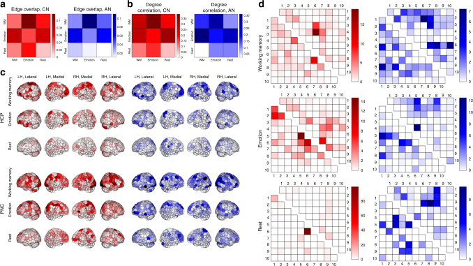
Fig. 2.

Model connections are widely distributed throughout the brain and demonstrate substantial overlap between models. a Edge overlap (number of shared edges normalized by the total number of unique edges in the models) between each pair of models within (off-diagonal) and between (main diagonal) data sets. In these and all subsequent matrix visualizations, HCP data are presented in the bottom triangle and PNC data are presented in the upper triangle. CN, correlated network; AN, anti-correlated network. b Spearman’s correlation of node degree between each pair of models both within (off-diagonal) and between (main diagonal) data sets. c Visualization of node degree for each model in the HCP (top three rows) and PNC (bottom three rows) data. CN degree is displayed in warm colors; AN degree is displayed in cool colors; darker color indicates higher degree. LH, left hemisphere; RH, right hemisphere. d Canonical networks that contribute disproportionately (i.e., value > 1; see main text) to each model. As in a and b, HCP models are represented in the lower triangles and PNC models in the upper triangles. Each number corresponds to one canonical network (Methods): 1 = medial frontal, 2 = frontoparietal, 3 = default mode, 4 = motor cortex, 5 = visual A, 6 = visual B, 7 = visual association, 8 = salience, 9 = subcortical, 10 = cerebellum. Models in a–c were generated with an edge-selection threshold of P < 0.01; models in d were generated with an edge-selection threshold of P < 0.001 for improved visualization and interpretability