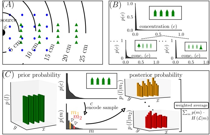
Fig 2. Overview of the analysis.

(A) shows the distance to the odor source for each of the locations of the two 16-location grid choices (green triangles and blue dots) and the imaged area. (B) shows probability distributions of the normalized odor concentrations (normalized by source concentration). The top panel shows the composite distribution, using data of all 16 locations, for the wide grid in the fast flow condition. Below are probability distributions for two selected locations (as indicated by solid green triangles in the inset). (C) Schematic of the information-theoretic analysis. On the left is the prior probability, which is equal for all 16 locations (depicted by equal height bars). The second column shows the composite distribution (top) and the result of discretizing it into M levels (bottom). The discretization recognizes that the observer has limited coding resources available. A sample from the discretized distribution results in an updated belief of where the observer is, represented by the posterior distribution. Two example posterior distributions are shown, one for drawing the sample m₁ (orange), and one for drawing the sample m₂ (red). Posterior distributions have lower entropy than the prior distribution, since the locations are no longer equally likely. The difference of the entropy of the prior and the weighted average of the posterior entropy is the information a navigator can expect to learn about location with a given sampling strategy. Note that this panel is a diagram for the analysis of encoding a single sample at a single time ($\mathcal{S}(n_{\text{bits}};1,1)$); an analogous strategy is used to analyze encoding with two sensors and/or encoding of multiple samples in time ($\mathcal{S}(n_{\text{bits}};r_{\text{spat}},r_{\text{temp}}$)).