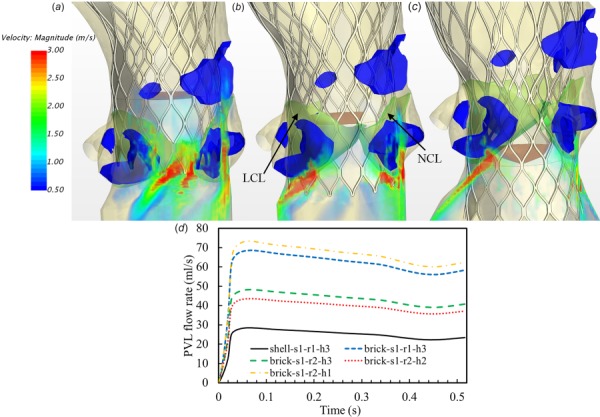
Fig. 8.

Volume rendering of velocity fields from the models with different deployment heights (a) higher than the optimum, h1 (brick-s1-r2-h1 model), (b) around the optimum, h2 (brick-s1-r2-h2 model), (c) lower than the optimum, h3 (brick-s1-r2-h3 model), and (d) corresponding PVL flow rate curves from five TAV models in Figs. 6–8
