. 2018 Jun 26;7:e36306. doi: 10.7554/eLife.36306

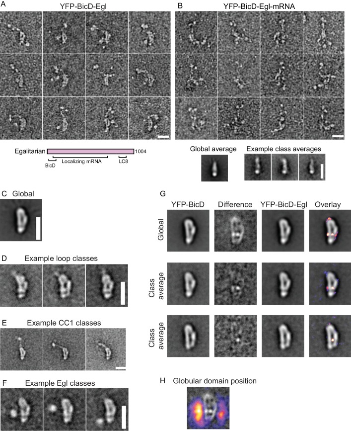
Figure 3. Electron micrographs of the YFP-BicD-Egl and YFP-BicD-Egl-mRNA complex.

(A) Montage of images showing that BicD retains the auto-inhibited looped conformation in the presence of bound Egl. A schematic of Egl (below) shows that the N-terminal domain binds BicD, the C-terminus binds dynein light chain (LC8), and mRNA binding is mediated through a large number (~800) of amino acids. (B) Montage of images showing that YFP-BicD no longer retains the auto-inhibited looped conformation in the presence of bound Egl and mRNA (K10min). Global and class averages are shown below the montage. (C) Average of all YFP-BicD-Egl molecules. (D) Example class averages of YFP-BicD-Egl with classification focused on the loop. (E) Example class averages of YFP-BicD-Egl with classification focused on the protruding YFP-CC1 region. (F) Example class averages of YFP-BicD-Egl with classification focused adjacent to the loop, to reveal the globular domain of Egl. (G) Co-alignment and classification of YFP-BicD and YFP-BicD-Egl. Upper row shows the average of YFP-BicD and YFP-BicD-Egl images (after an initial alignment, classification and selection of particles in similar orientations). Difference maps are shown in the second column and the difference map is overlaid as a heatmap onto the average of YFP-BicD-Egl in the fourth column, to show clearly the locations of greatest difference. Second and third rows show the averages and differences for individual classes. See Figure 3—figure supplement 5 for the full classification. (H) Heatmap showing the position of the globular Egl domain. Scale bars = 20 nm.

Figure 3.

Figure 3—figure supplement 1. SDS-PAGE gels of Egl.
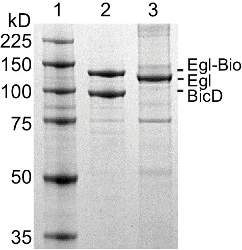
Figure 3—figure supplement 1.

(lane 1) Molecular mass markers, (lane 2) BicD co-expressed with Bio-tagged Egl, (lane 3) Egl expressed alone. 4–12% SDS-gel, MOPS buffer.
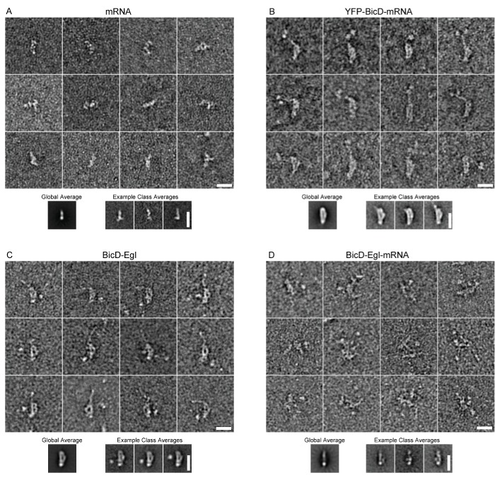
Figure 3—figure supplement 2. EM of other conditions imaged in this study.

Figure 3—figure supplement 2.

(A) Montage showing example raw images of mRNA (K10min). Global average and example class averages are shown below the montage (n = 2039). (B) Montage showing example raw images of YFP-BicD-mRNA. Global average and example class averages are shown below the montage (n = 1393). (C) Montage showing example raw images of BicD-Egl. Global average and example class averages are shown below the montage (n = 3697). (D) Montage showing example raw images of BicD-Egl-mRNA. Global average and example class averages are shown below the montage (n = 3526).
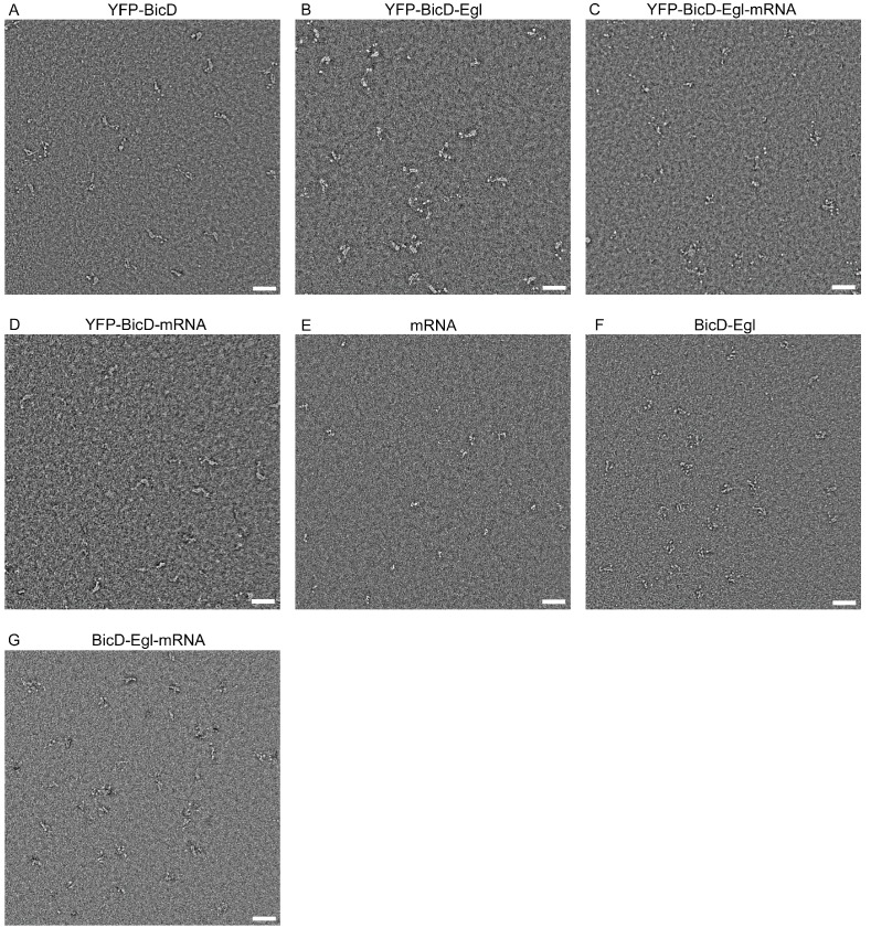
Figure 3—figure supplement 3. Fields of view of all conditions imaged in this study.

Figure 3—figure supplement 3.

Scale bars = 50 nm.
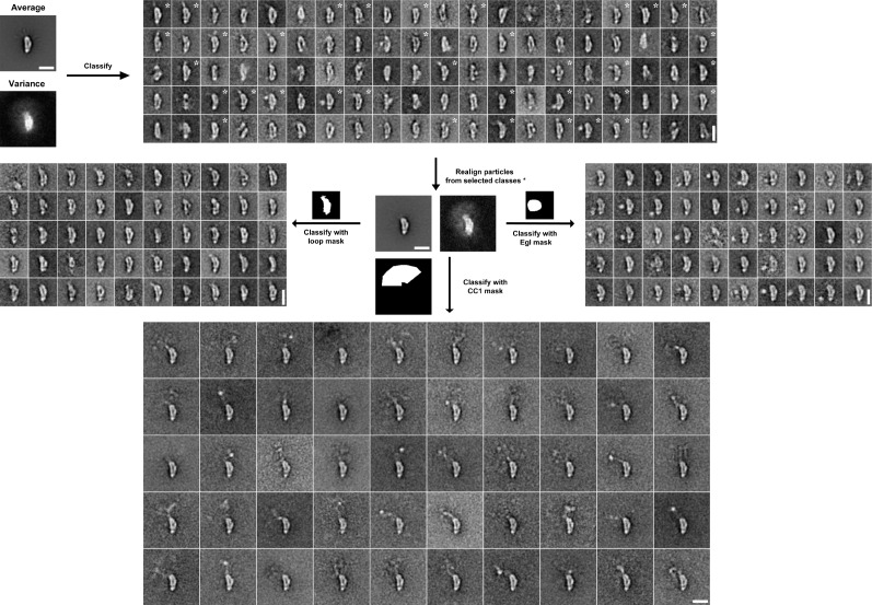
Figure 3—figure supplement 4. Image processing scheme for YFP-BicD-Egl EM data.

Figure 3—figure supplement 4.

Following initial alignment of the full dataset (n = 4117), images were classified into 100 classes using a variance mask. Classes in similar orientations were selected (based on the appearance of class averages and class variances, asterisks show selected classes). Particles from selected classes were re-aligned (n = 1488). Aligned images were classified into 50 classes using masks around the loop, the protruding YFP-CC1 region or the region adjacent to the loop, in order to reveal the Egl globular domain. Scale bars = 20 nm.
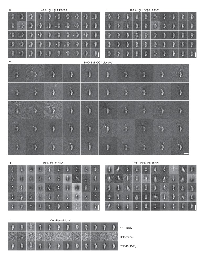
Figure 3—figure supplement 5. Other classifications used in this study.

Figure 3—figure supplement 5.

(A) Classification of BicD-Egl using a mask adjacent to the loop to reveal the globular domain of Egl. (B) Classification of BicD-Egl using a mask around the loop. (C) Classification of BicD-Egl using a mask around the protruding CC1 region. (A), (B) and (C) are classifications of re-aligned images (n = 1765) following an initial alignment (n = 3697) and selection of classes in the most common orientation. (D) Classification of BicD-Egl-mRNA (n = 3526). Scale bars = 20 nm. (E) Classification of YFP-BicD-Egl-mRNA (n = 3345). (F) Classification of combined YFP-BicD and YFP-BicD-Egl datasets (most common orientation only). Central row shows difference images between the two datasets. Scale bars = 20 nm.