Appendix 5—figure 1. The population variance of clock states is reduced by dusk and can be computed geometrically.

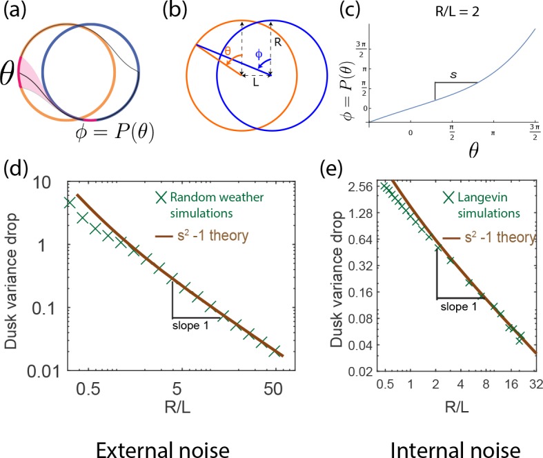
(a) A population of clocks near state ${\displaystyle \theta }$ on the day cycle is mapped to the neighborhood of state ${\displaystyle \varphi }$ on the night cycle by the dusk transition. We define ${\displaystyle \varphi =P(\theta )}$ to be the map relating the clock state ${\displaystyle \theta }$ on the day cycle just before dusk to its eventual position ${\displaystyle \varphi }$ on the night cycle after dusk (assumed greater than the relaxation time). (b) This map can be analytically computed for circles of size R with centers separated by length L. (c) For a given R/L = 2 , we obtain ${\displaystyle P(\theta )}$ shown here. Since ${\displaystyle \theta =\pi /2}$ corresponds to the dusk time of the entrained trajectory, the slope ${\displaystyle s^{-1}=dP/d\theta }$ at ${\displaystyle \theta =\pi /2}$ determines the change in population variance of clock states at dusk. (d,e) The variance drop ${\displaystyle s^2}$ at dusk, defined as ${\displaystyle {\sigma }^2\to {\sigma }^2/s^2}$ at dusk, seen in both the external (averaging over weather) and internal noise (averaging over Langevin noise) simulations agree well with the geometrically computed ${\displaystyle s(R/L)}$, especially at large ${\displaystyle R/L}$. We find that ${\displaystyle s^2-1\sim L/R}$ for large-${\displaystyle R/L}$ limit cycles.