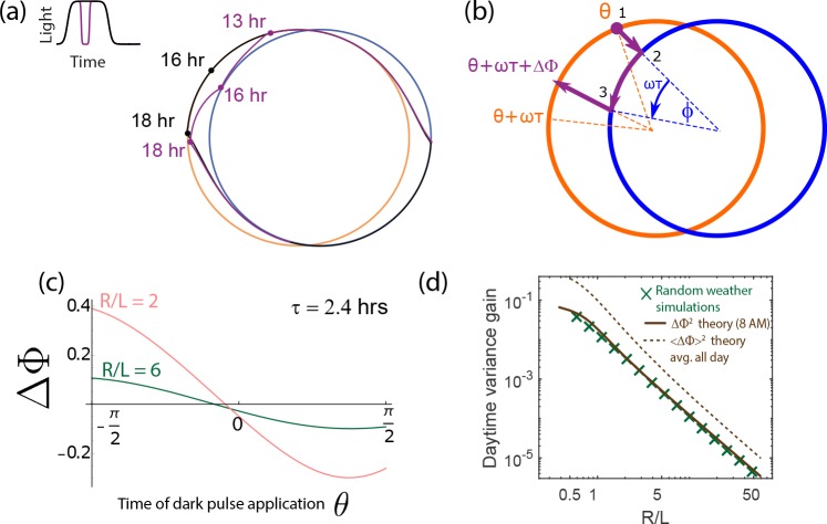
Appendix 5—figure 2. Increase in population variance due to random weather conditions can be estimated from the phase shifts ${\displaystyle \mathrm{\Delta }\mathrm{\Phi }}$ due to dark pulses (i.e., the Phase Response Curve).

(a) A single dark pulse administered during the day shifts the phase of a clock (purple) relative to a clock that experiences no such dark pulse (black). (b) We can compute the phase shift ${\displaystyle \mathrm{\Delta }\mathrm{\Phi }}$ due to such a dark pulse geometrically by computing the deviation in trajectory. Assuming a dark pulse of length ${\displaystyle \tau }$, the clock evolves for a time ${\displaystyle \tau }$ according to the night cycle dynamics. At the end of such a pulse, we switch back to the day limit cycle and compute the resulting phase shift ${\displaystyle \mathrm{\Delta }\mathrm{\Phi }}$. (c) The resulting phase shift ${\displaystyle \mathrm{\Delta }\mathrm{\Phi }}$ due to a pulse of length ${\displaystyle \tau =2.4}$ hrs, depends on the time $\theta$ when it is administered but is generally smaller for larger ${\displaystyle R/L}$. (d) We find that ${\displaystyle \mathrm{\Delta }{\mathrm{\Phi }}^2}$ for a specific ${\displaystyle \tau =2.4}$ hrs dark pulse administered at the same time (8 AM) falls as ${\displaystyle (L/R{)}^2}$ for large-${\displaystyle R/L}$ limit cycles. This trend matches the variance gain ${\displaystyle {\sigma }_{clouds}^2}$ seen in stochastic simulations that average over random weather conditions (pulses of different length, intensity and time of application). The broken brown curve shows a theoretical prediction for such an average ${\displaystyle ⟨\mathrm{\Delta }{\mathrm{\Phi }}^2⟩}$, obtained by sampling the curve shown in (c) at different points of application and differing intensity. Despite the presence of a variance-reducing zero around mid-day in (c), ${\displaystyle {\sigma }_{clouds}^2}$ drops as ${\displaystyle (L/R{)}^2}$, much as ${\displaystyle \mathrm{\Delta }{\mathrm{\Phi }}^2}$ for any particular pulse. (Brown theory curves translated together using one fitting parameter).